Clip Art

Now it is Time to have Fun with Excel

Since you have worked so hard with the Basic Concepts in Excel I figured that it is time to show you some of the fun side of Excel.

Yes it is true you can have fun…

Working with Clip Art

Most computers have Clip Art built into the programs such as Microsoft Office, however, there are a few companies and the military and government organizations that like to save space by not adding the Clip Art portion of the program in. So if you are using a computer supplied by one of the above mentioned you will be able to read the steps but you will not be able to work through them.

I know that I am not going in order of the buttons in the Illustrations Group on the Insert Tab.

Clip Art

What makes Clip Art different from other images such as Pictures?

Clip Art basically are the images that look more cartoonish, hand drawn, and charactertures, you know when the artist has drawn a person and their head is too big for their body.

If you have not already done so go ahead and open an Excel Workbook. Then go to the Insert Tab on the Ribbon, there you will find a Group called Illustrations. You should see four buttons that you can choose from.
1. Picture – you can go anywhere on your system or network to find Pictures and import them into Excel.

2. Clip Art – this should bring up a selection of Clip Art that you can choose from. There are places that you can go to online and find many more collections of Clip Art. Be careful doing this because there are some web-sites that have viruses on them.

3. Shapes – you can choose from a large selection of shapes if you desire to create something for yourself. This can be done by using multiple shapes and arranging them how you want. Latter I will show you how to make a quick robot with Shapes.

4. SmartArt – this is a cool addition to the Excel program, you used to have to build these from scratch, or the ground up. I have a complete lesson on this latter in the Intermediate Concepts Section.

The Clip Art Button

When you click the Clip Art Button you will get a Dialog Box to open up. The Clip Art Dialog Box will have five sections to it.

1. Search For – if you have a specific item that you are looking for you can type it in the Search For Text Area then click the Go Button. In the Large white area below it will show you what if found that matched your criteria.

2. Search In – This section has a list of different places that you can find Clip Art. If it does not say All Collections use the drop down arrow and make sure that all the boxes are checked.

3. Results Should Be – here you can tell Excel what you want it to search for. Although the Photographs, Movies, and Sounds are not technically clip art.
     a. Clip Art
     b. Photographs
     c. Movies
     d. Sounds

4. The View Area – this is where the results of the search will appear.

5. The Three Buttons in the bottom
     a. Organize clips – here is where you can go if you have downloaded Clip Art from the internet, you can                  add them to the folder that you wish them to be in or you can create your own folders.
     b. Clip art on Office Online – this will take you to the Microsoft Office Online site where you can pick and choose from their selection of Clip Art.
     c. Tips for finding clips – this will take you to the Excel Help Screen.

Inserting Clip Art into your Spreadsheet

There are three ways that you can insert Clip Art into your Spreadsheet. After you have searched for the Clip Art that you wish to add;

1. The Double Click Method – you can click the Left Mouse Button twice and the Clip Art that you Double Clicked on will be placed into your Spreadsheet.

2. Drag and Drop – you can hover over the Clip Art that you wish to insert into your Spreadsheet and Hold the Left Mouse Button down and drag the Clip Art to where you wish to place it and let go.

3. The Drop Down Arrow – as you hover over the Clip Art that you want to insert into your Spreadsheet you will see a grey button appear down the right hand side of the Clip Art sample. If you Click on the Button you will get a Dialog Box that allows you to choose from several choices. When this Dialog Box appears you can choose Insert and it will put the selected Clip Art into your Spreadsheet.

4. Okay, so I misled you… There are actually four ways to add Clip Art, if you get the Dialog Box you can choose Copy and then Paste it into the Spreadsheet.

Suggestions

I would like to take this opportunity to ask the readers what they would like to see posted in this blog.

Please tell me what version of MS Office that you use and what program, Excel, Word, PowerPoint, etc.

Also, if you could ask questions or make comments about what you would like to see in an instructional book, what would it be.

Let me know, you can either leave a comment or email me at shawnrblogs@gmail.com

Thank you.

The Easiest Way to Create a Chart

     Have someone else do it...

     Just kidding.

The Easiest way to Create a Chart

Okay, are you ready for the Easiest way of Creating a Chart?

Well, I hope that you are because I am going to give it to you even if you do not want it.

The First thing that you need to do is to select the Data Range for your Chart. I would like you to select the Range of Cells from A5 to G13.

No w that that is done.

Now, you have two hands, Right?

Ten fingers or perhaps you may say no I have eight fingers and two thumbs.

Hold your hands up, either hand I want you to choose one finger, not the third finger over from either direction…

Some people get that joke right away, makes me wonder do they use that finger a lot…

There is the Functions Button Row on your Keyboard, the F1, F2, F3, F4, all the way to F12. It is usually the upper most row of Buttons on the Keyboard. They are actually good for something other than catching dust. Well I want you to use the finger that you chose and click the F11 Button.

Ka-pow…

Two things should have happened simultaneously Excel should have created a Tab Called Chart1 and it also created the Chart.

Did I lie, was that not the easiest way that you created a Chart?

Okay, I would like for you to go back to the Charts Tab and this time Select Cells A5 to G5 and Cells A15 to G15. It should look something like the below picture. Then use the F11 Key again.

You should get a Second Chart on a Chart2 Tab. Now you have the option of showing the Boss both charts in an uncluttered Spreadsheet. Or you could have something that looks like this. Which looks best to you, the three Tabs or the One Tab with all the information on it?

What choice is the easiest to read, especially for the audience?

Charts the Easier Way

     NOTE: The Contextual Tabs are called Contextual because they appear in context of what you are dealing with. So with Charts you will get the Design, Layout, and Format Tabs that deal with Charts. If you are working with Pictures then you will get the Contextual Tab that deals woth Pictures.
   
     The Easy to Create a Chart

     If you want to create a Chart that has the Total, select Cells A5 to G5, than hold your CTRL Key down and select Cells A15 to G15. Then go to the Insert Tab and click the Column Button in the Charts Group. Once the Dialog Box appears click the 2-D Clustered Column Chart, or the first one in line and you will get the same Chart that you had before. With the Chart Selected you will get the Contextual Tabs once again.

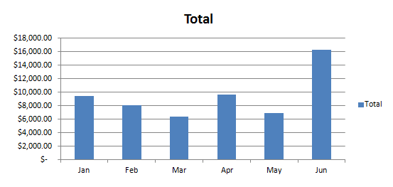
Your Chart should look like this.

     Now then go ahead and Delete this Chart. I know, it is not fair, I keep having you make the Charts and then Delete them, well practice makes perfect. As they say, but who are they, I have always wondered.

     This time I am going to have you create a Chart with different information in it. Select the Cell Range A5 to G13, you can do this a couple of different ways. One way is to Click into Cell A5 and then hold your Left Mouse Button down and drag to Cell G13 and then let go. Another way to do this is to Click into Cell A5 and then hold your Shift Key Down and Click into Cell G13, then release your Shift Key.
Now, you know where to go and what to do. Hey, I mean go to the Insert Tab, what were you thinking…

     Once you get to the Insert Tab use the Column Button and choose the First Button in the 2D Column List called Clustered Column. Now your Chart should look like this.

     This time you have a list of Items in the Legends area, the Category or Horizontal Value is not the Product Name, the Values are still in Dollar Format like the Totals. This time, however, you have several different Colors for the Months instead of just one Color as with the Totals. This way it is easier to keep the Product Totals for the Months separated and quickly readable.

     I bet you know what I am going to ask you to do now, please Delete the Chart. Because it is almost time to learn the quickest way to create a chart that I know of.

Charts the Hard Way

To follow the steps in this you will need to download this file Basic Concepts it has been designed for Excel 2007

The Hard way to Create a Chart

                With the Charts Spreadsheet being the active sheet go to the Insert Tab and there is a group called Charts.  This Group has several kinds of Charts that you can choose from.  There are Column Charts, Line Graphs, Pie Charts, Bar Charts, Area Charts, Scatter Charts, and Other Charts.  The Most common and universal Chart is the Column Chart.  This is the one that you will be spending most of your time working with.

                When you click the Column Button a Dialog Box will open and it has several different styles of Column Chart that you can use.  The most common Chart in this Dialog is the 2-D Clustered Column Chart, or the first one in line.

                Click on the 2-D Left most Button and two things will happen.  The First thing that most people notice is that there is now a blank box covering part of your data.  The second thing, sometimes this needs pointed out before people notice, is that there are now three more Tabs on the Ribbon.  They are Design, Layout, and Format.

                You can move the Empty Box around on the Spreadsheet so that you can see all of you data.  As you hover over the Blue Surround of the Box you will see the Crossed Arrows, when you get this symbol hold your Left Mouse Button down and move the Box to where you want it.  There are also Eight sets of three dots, one in each corner, and one in the middle off each of the runs, these can be used to make the Chart larger or smaller.  As you hover over the three dots your cursor will change from the crossed arrows to either a two headed arrow pointing up and down, a two headed arrow pointing right and left, or a two headed arrow pointing at a diagonal.  Then you can hold your Left Mouse Button and drag the direction of the arrows to resize your Chart.

                With that said, how do you get your chart to show information?

                On the Design Tab there is the Data Group and in the Data Group there is a button called Select Data.  Click this Button and a Dialog Box will appear, it has the title Select Data Source.

  In the Chart Data Range it will automatically choose the Cell that your Cursor is in at the moment.  As long as you can see the black around white text all you have to do is select where you want the information to be pulled from.  Select Cells A5 to G16, you will see the Dancing Ants around the selected area.  You will also see =Charts!$A$5:$G$16 in the Chart data range text box.  Also there will also be information in the Legend Entries (series) section and the Horizontal (Category) Axis Label section.  Now Click OK.

                Is this more like what you expected?

                I tend to think that there is too much information in the Chart now.  Do you?

                That is okay because you can deal with that, as soon as I show you how that is.

                The first thing that you need to do is figure out what information it is that you want to see.  Do you want to see just the Totals or Just the Item information?

There are two ways that you can accomplish this task, I will show you how to do both.

             For now I will show you how to just show the Totals for the months.  The first thing that you need to do is go back to the Select Data Button, which is on the Design Tab in the Data group.

             There are a couple of ways that you can get the exact information that you want.  One way is slightly easier than the other.

                The first way that I will show you is working inside of the Select Data Source Dialog Box.

Months in the Legend

Product s in the Legend

                There is a button in the middle of the Dialog Box, it says Switch Row / Column, press this button and your information will change sides as seen in the sample above.  Once this is done, you can now remove the information that you no longer want or need.

                Click onto the White Bread so it has the Blue around it and press the Remove Button, continue to hit the Remove Button until the only items left are Total and Average, then remove Average.

                Now click the Switch Row / Column Button again and then click OK.  Now you should have a Column Chart that has the Totals in the main area and the Months in the Legend.  Notice that the Colors are corresponding, January is Purple, February is Dark Blue, etc, etc…

                Have you noticed that the data used to create the Chart has a Green Box around the Legend Information, a Purple Box around the Label “Total”, and a Blue Box Around the Data for the Totals.

                Now that you know how to get the information that you want the hard way I’ll walk you through getting the information an easier way, use the Undo Button, it is on the Quick Access Toolbar it looks like an Arrow that is Hooked to the Left, or you can use the CTRL + Z Buttons on the Keyboard.

                Now that you have the blank Chart once again, make sure that the Chart is still active; you will know that is active if you still have the Three Additional Tabs on the Ribbon.

                On the Design Tab click the Select Data Button and then use the Backspace Key, this should clear the Chart Data Range portion of the dialog box.  Hover over Cell A5 and hold your Left Mouse Button down and pull to Cell G5 then let go.  The Chart Data Range should now read =Charts!$A$5:$G$5.  Now hold your CTRL Key down and hover over Cell A15.  Once you are hovering over Cell A15 continue to hold the CTRL Key down and hold Your Left Mouse Button down and move to Cell G15.  The Cart Data Range should now read =Charts!$A$5:$G$5,Charts!$A$15:$G$15, click the OK button and you will see the Legend now says Total and you have the months Jan to June as the Labels for the Columns.

                Congratulations, you now know the Hard Way to create a Chart.

                There are some people who prefer to create the Charts this way.

                I am going to have you Delete the Chart now, click onto the Blue Border or the Chart and use the Delete Key.  By clicking the Blue Border you will ensure that the Chart has been selected instead of one of the objects inside of the Chart.

Chart Objects in Excel 2007

Chart Object, What they are

                The Objects are the Vertical Axis or Values, Chart Title, Series Legend Entry, Horizontal Axis or Category, Series Total, and many other portions (objects).

                Click on the Blue Surround that will make sure that the Chart is selected as opposed to one of the Objects within the Chart. 

                If you hover over the White Area, where the Blue Boxes are this is the Chart Area object.

                If you hover over the Grey Lines inside of the Red Box they are the Vertical Axis Major Gridlines, they are associated with the Numbers at the Left or the Values and the Columns. 

                If you hover over the White Area within the Red Box, this is called the Plot Area.

                The Object in the second sample in the Black Box is the Vertical Access (Value).

                Inside the Red Box is the Chart Title.

                The Object in the Green Box is the Legend.

                The Object in the Purple Box is the Horizontal Axis (Category).

            These Objects will change as to the information that you have in your Chart.  If you have the Product as opposed to the Months then the Objects will reflect the Product information.  There are also ways that you can manipulate the Objects, Change the Color, Change the Background Color or add a Picture.

                I will show you how to do all of this later on in the Charts Lesson in the book.

Renaming Spreadsheets Excel 07

     You can rename the Tabs from Sheet1 to whatever You desire.  There are two ways that You can accomplish this task;

     Double Click, this one takes some practice you will have to click the Tab twice at the correct speed.

     Right Mouse Click, this is an easier way to accomplish the task.  One right Mouse click on the Tab that you wish to rename.

     Let us practice renaming the Tabs.  Make sure that Sheet1 is the Active Tab, I know that it is Active because it is white in color and has no line dividing it from the Spreadsheet.  Let’s name it Phonebook; you can try either way to rename the Tab that you want, Double Click or Right Mouse Click.  Once you have renamed it either move the cursor to somewhere on the Spreadsheet and Left Mouse Click or hit the Enter Key and this will finish the Rename process.

     Now let us click to Sheet2, and you will rename this to Address Book.

     That is all there is to it, of course you can change the names to whatever you desire.

Questions to the readers

I am currently writing an e-book on Excel, what concepts would you like to have explained?

What Version of Microsoft Office do you use?

Please let me know either by shawnrblogs @ gmail.com  remove the spaces before and after the @, or by comments.

The Quick Access Toolbar in Excel 07

The Quick Access Toolbar is located to the right of the Microsoft Office Symbol and Above the Home Tab.
Right out of the box, initial install, there are three buttons by default; Save, Undo, and Redo. If you want to you can add buttons or remove buttons from the Quick Access Tool Bar. There are a few of ways that we can do this.

The Quick Access Toolbar Button

     To the right of the Quick Access Toolbar there is a symbol that looks like a line above a triangle that is pointing down, this is actually a button.
   
     When you press the button a dialog box appears. With this dialog box you can add or remove buttons from a standard list. As you can see there are some that have a check-mark to the left of them. These are the buttons that will show in the Quick Access Toolbar.

     To add more buttons just click on the word, for instance New, This will add the New Spreadsheet Button to the Quick Access Toolbar; the Dialog Box will close after you click. If you want to add more of the predefined buttons then you can repeat the same steps as often as you want.

     To remove the button from the list, simply click on the name of the button that you wish to remove from the Quick Access Toolbar and the check-mark will be removed, the Dialog Box will close, and it will remove the button from the Quick Access Toolbar.

     There are three other buttons on the Customize Quick Access Toolbar; they are More Commands, Show Below the Ribbon, and Minimize the Ribbon.

More Commands

     The More Commands Button will open another Dialog Box; this dialog box has many options for
customizing Microsoft Excel. I will talk about most of them later on in the book. For now I will discuss
the Customize the Quick Access Toolbar, in the Customize Section.

     This Dialog Box is split into many parts; On the right side we have a list of sections that we can
access, there is the Choose commands from drop down, below that we have the command buttons for
that particular command group. Below that we have the Show Quick Access Button Below the Ribbon
check box. Next we have the Add and Remove Buttons. Then the Customize Quick Access Toolbar drop
down, here we can choose if we want to apply the changes in the Quick Access Toolbar to all Documents
or just this particular Spreadsheet. Below that we have a list of the buttons that will appear in the Quick
Access Toolbar. Then we have the Reset Button which will reset the Quick Access Toolbar to the default
settings. The Modify Button applies to special buttons that you can create for Macros, we will talk about
these later. To the right of the button list there are two buttons that we can use to change the order of
the buttons on the Quick Access Toolbar, the closer the button is to the top of the list the closer to the
Office Symbol it will be. We then have the OK and Cancel buttons. If we made changes to the list we
need to click the OK button for those changes to take effect, if we use the Cancel button it will not keep
the changes that we have just made.

Add a Quick Access Button from a Group

     There is another way to add a button to the Quick Access Toolbar using the right mouse button.
If you want to add the Insert Picture Button, go to the Insert Tab, right mouse click on the Picture Icon
and click the Add to Quick Access Toolbar.

Show Below the Ribbon

     The Show Below the Ribbon, option will move the Quick Access Toolbar from the default location to bellow the ribbon.  When you do not know that this is a feature and someone has moved the Quick Access Toolbar it is hard to find. I know because before I realized that this was an option it happened to me.
When the Quick Access Toolbar is below the Ribbon the choice changes to Show Above the Ribbon.

Minimize the Ribbon

     The Minimize the Ribbon is another option that Microsoft has given. When you use this option
the Workbook area becomes larger. This is an option that Microsoft did not advertize. I learned about
this option when I was told that I was going to be sowing others how to use Microsoft Office 2007.
There was no training that neither I nor my boss received.

     The program was installed on one computer in my classroom; someone had accidentally removed the Ribbon before either of us had seen the new program. It took awhile but my boss figured it out and informed me as to how to fix it.

     To Minimize the Ribbon with the control button, click the Button and then click on the last choice, Minimize the Ribbon. See the picture to the right. With the Ribbon Minimized to see the groups on the ribbon just click on the tab name such as Home, Insert, Page Layout, etc…

     To maximize the Ribbon you can click on the Quick Access Toolbar Button again and uncheck the Minimize the Ribbon. This will restore the Ribbon to its original state.

The Quick Access Toolbar Right Mouse Click 

     With a quick click or the Right Mouse Button you can remove a button from the Quick Access Toolbar, all you have to do is Right Mouse Click the Icon and use the Remove from Quick Access Toolbar.

The Alt Key

NOTE: You can use either lower case or upper case letters. It may take a bit longer but it works.

If for some reason your mouse dies these is still a way that you can navigate the Excel Workbook. That way is the Keyboard. By pressing the ALT Key Numbers and Letters appear. By pushing the corresponding key you can Navigate

1. F – will open the Office Symbol Dialog Box
2. 1 – The First Button on the Quick Access Tool Bar
3. 2 – The Second Button on the Quick Access Tool Bar
4. 3 – The Third Button on the Quick Access Tool Bar
5. H – will display the Home Tab
6. N – will display the Insert Tab
7. P – will display the Page Layout Tab
8. M – will display the Formulas Tab
9. A – will display the Data Tab
10. R – will display the Review Tab
11. W – will display the View Tab
12. L – will display the Developer Tab
F will open the Office Symbol Dialog Box

Once the F or Office Symbol Dialog box opens there will be other choices. After you make a single choice the Dialog will close. If you want to do something else you will need to go through the motions again.

1. N – will open a New Spreadsheet
2. O – will open the Open Dialog Box
3. S – will Save the Workbook
4. A – will open the Save As Dialog Box
5. F – will open up the Save As Choices
6. P – will open the Print Dialog Box
7. W – will open the Print Choices
8. E – will open the Prepare Choices
9. D – will open the Send Choices
10. U – will open the Publish Choices
11. C – will Close the Spreadsheet
12. I – will display the Excel Options Dialog Box
13. X – will Exit the Excel Program

1  –  The First Button on the Quick Access Tool Bar. If the Save Button is the first button, by default on install, then the number 1 will Save the Workbook.
2 – The Second Button on the Quick Access Tool Bar.  If the Undo Button is the first button, by default on install, then the number 2 will Undo the last modification made to the Workbook.
3 –  The Third Button on the Quick Access Tool Bar,  If the Redo Button is the first button, by default on install, then the number 3 will Redo the last Undo made to the Workbook.

H will display the Home Tab

There are two ways to Navigate the Submenus, to Navigate you can either press the letter associated with the ALT Tab or you can use your Arrow Keys. If you are in one of the Menus the ESCAPE Key will go back one level.

The Clipboard Group

1. V will bring up the Paste Menu
     a. P – for Paste
     b. F – for Formulas
     c. V – for Paste Values
     d. B – for No Borders
     e. T – for Transpose
     f. N – for Paste Ink
     g. S – for Paste Special
     h. H –for Paste as Hyperlink
     i. A – for As Picture
          i. C – for Copy as Picture
          ii. U – for Past as Picture
          iii. I – (the capital i) for Paste Picture Link
2. X – to Cut a selected area
3. C – to Copy a selected area
4. FP – to copy the Format from a selected area
5. FO – will bring up the Clipboard Dialog

The Font Group

6. FF – will open the Font Face Dialog
7. FS – will open the Font Size Dialog
8. FG – is the command to take the Font Size up one size
9. FK – is the command to reduce the Font Size one size
10. 1 – will Bold the selected area
11. 2 – (The number 2) will Italicize the selected area
12. 3 – (The Number 3) will Underline the selected area
13. B – will add Borders to the selected area
14. H – will bring up the Cell Background Color Dialog
15. FC – will bring up the Font Color Dialog
16. FN – will Bring up the Format Cells Dialog Box – Font Tab

The Alignment Group

17. AT – Top Align
18. AM – Middle Align
19. AB – Bottom Align
20. FQ – Orientation, or test angle
21. W – Wrap Text
22. AL – Align Left
23. AC – Align Center
24. AR – Align Right
25. 5 – Decrease Indent
26. 6 – Increase Indent
27. M – Merge and Center
28. FA – will bring up the Format Alignment Dialog Box – Alignment Tab

Number Group

29. N – will bring up the Number Dialog Box
30. AN – will bring up the (Accounting Number Format) Currency Dialog Box
31. P –Percent Style
32. K – Comma Style
33. 0 (Zero, the number not the letter) – Decrease Decimal
34. 9 – Increase Decimal
35. FM - will bring up the Format Number Dialog Box – Number Tab

The Style Group

36. L – Opens the Conditional Formatting Dialog Box
37. T – Opens the Format as Table Dialog Box
38. J – Opens the Styles Dialog

The Cells Group

39. I – Opens the Insert Dialog Box
40. D – Opens the Delete Dialog Box
41. O (ooh, the letter not the number) – Opens the Format Dialog Box

The Editing Group

42. U – Opens the AutoSum Dialog Box
43. FI (I capitol i) – Opens the Fill Dialog Box
44. E – Opens the Clear Dialog Box\
45. S –Opens the Sort & Filter Dialog Box
46. FD –Opens the Find & Select Dialog Box

You can do the same for all the Tabs and Groups within Excel.

Navigating a Spreadsheet Part 1

Remember: The size of the Scroll Bars will vary with the amount of information held Within the Workbook.

Navigating a Spreadsheet,

There are several ways in which to Navigate a Spreadsheet.

The Scroll Bars

1. Vertical Scroll Bar, this allows us to move up and down the Spreadsheet. It is located
at the right hand side of the Workbook Window.

2. On the Vertical Scroll Bar there are two Arrows, one on top and the other on the
bottom. You can use these to Scroll Up and Down The Top Arrow will move the
Spreadsheet towards the Top or Row 1, the Bottom Arrow will move the Spreadsheet
towards the bottom or towards row 1048576.

3. The Horizontal Scroll Bar, This is located at the bottom of the Workbook just above the
Status bar and to the right of the Tabs.

4. The Horizontal Scroll Bar has two arrows at either side of it. The one to the left will
scroll back towards Column A, the one on the right will scroll towards Column XSD (the
last Column in the Spreadsheet)

The Mouse Wheel

1. If you have a Wheel Mouse you can push down on the wheel you will get a Four Pointed arrow, this will allow you to move any direction on the Spreadsheet that you >want. One thing about this that I have discovered is that if you want to scroll down quickly, before you click the wheel, get close to the top of the Spreadsheet Cells. Then after you click the wheel the closer you get to the bottom of the Spreadsheet the faster it will scroll down.
The wheel also moves you up and down the Workbook, if you roll the wheel forward it will take you towards the top of the Spreadsheet, Row 1. If you roll the wheel backwards it will move the Spreadsheet down, towards Row 1048576.

The Mouse Left Button

1. Take your Mouse and hover over any Cell then click the Left Mouse Button and it will put you into that cell

The Tab Key

1. The Tab Key will take you one Cell to the right
2. SHIFT + Tab will take you one Cell to the left

The Enter Key

1. The ENTER Key will take you one Row down
2. SHIFT + ENTER will take you one Row up

The Address Bar

1. Will take you to the Cell Address that you tell it to
     a. Once you enter the Cell Address hit Enter

The Arrow Keys

1. Up Arrow will take you one Cell up
2. Down Arrow will take you one Cell Down
3. Left Arrow will take you one Cell to the Left
4. Right Arrow will take you one Cell to the Right

CTRL + Arrow Keys (Assuming you are starting from Cell A1 with information to cell H35)

1. First use of CTRL + Down Arrow will move you to Cell A35
2. Second use of CTRL + Down Arrow will move you to Cell A 1048576
3. Firs t Use of CTRL + Up will move you to Cell A35
4. Second use of Up Arrow will move you to Cell A1
5. First use of CTRL + Right Arrow will move you to H1
6. Second Use of CTRL + Right Arrow will move you to Cell XFD
7. First use of CTRL + Left will move you to Cell H1
8. Second use of CTRL + Left Arrow will move you to Cell A1

CTRL + Arrow Keys (Assuming you are starting from Cell A1 with information to cell H35 with missing information in Cell A14 and missing information in Cell E1)

1. First use of CTRL + Down Arrow will move you to Cell A13
2. Second use of CTRL + Down Arrow will move you to Cell A15
3. Third use of CTRL + Down Arrow will move you to Cell A35
4. Fourth use of CTRL + Down Arrow will move you to Cell A 1048576
5. Firs t Use of CTRL + Up will move you to Cell A35
6. Second use of Up Arrow will move you to Cell A15
7. Third Use of CTRL + Up will move you to Cell A13
8. Second use of Up Arrow will move you to Cell A1
9. First use of CTRL + Right Arrow will move you to D1
10. Second Use of CTRL + Right Arrow will move you to Cell F1
11. Third use of CTRL + Right Arrow will move you to H1
12. Fourth Use of CTRL + Right Arrow will move you to Cell XFD
13. First use of CTRL + Left will move you to Cell H1
14. Second use of CTRL + Left Arrow will move you to Cell F1
15. Third use of CTRL + Left will move you to Cell D1
16. Fourth use of CTRL + Left Arrow will move you to Cell A1

Go To

With the Go To you can navigate to any Cell in the Spreadsheet that you want to, similar to the Address Bar. The quick way to get to Go To is CTRL + G.

The fx is a Button and Functions Dialog Bar

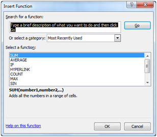
     The fx is not only there to tell you that the Function Dialog bar is coming up next, it is actually a button. Once you press this symbol you will get a dialog box that gives you several choices of prebuilt functions that Excel has. I will talk more at length about these later. I will also explain the parts of the dialog box later.

     There are also a few more ways that we are able to access the Functions Dialog box, using the Auto-sum button or it can be accessed from the Formulas Tab. I will go into depth about these choices later.

     The Function Dialog Bar shows the function as opposed to the total that is shown by default in the Workbook Cell. As we see here in cell A4 we see 3200, yet in the Functions Dialog Bar we see =SUM(A2:A3) or the actual Function its self.










    If the Function is longer than the functions dialog box the code for the function will wrap around much the same as a paragraph in Microsoft Word. Two arrows will appear at the right side of the screen just to the left of the double chevron. If you use the single arrows you can scroll up or down one line at a time. If you use the double chevron it will expand the Functions Dialog Bar and show several lines.





Normal Function Dialog View


Expanded Function Dialog View

      The position of the arrows will change slightly from the collapsed view of the Functions Dialog Box, instead of being beside each other as in the previous example. In the expanded view the buttons are stacked.

One Important Note about Excel

     Working with Excel will become easier once you realist that EXCEL DOES NOT CARE ABOUT YOU. Excel is considered the SNOB of the Microsoft Office Suite. The only things that Excel cares about are numbers, and numbers are the only thing. Not you, not text, or labels as Microsoft calls them. Not even other Excel Workbooks.


     Excel has been set up to automatically by default have text to the left of the Cell and numbers to the right of   the Cell.

The Quick Access Toolbar

The Quick Access Toolbar is located to the right of the Microsoft Office Symbol and Above the Home Tab.
Right out of the box, initial install, there are three buttons by default; Save, Undo, and Redo. If you want to you can add buttons or remove buttons from the Quick Access Tool Bar. There are a few of ways that we can do this.

The Quick Access Toolbar Button

To the right of the Quick Access Toolbar there is a symbol that looks like a line above a triangle that is pointing down, this is actually a button.

When you press the button a dialog box appears. With this dialog box you can add or remove buttons from a standard list. As you can see there are some that have a checkmark to the left of them. These are the buttons that will show in the Quick Access Toolbar.

To add more buttons just click on the word, for instance New, This will add the New Spreadsheet Button to the Quick Access Toolbar; the Dialog Box will close after you click. If you want to add more of the predefined buttons then you can repeat the same steps as often as you want.

To remove the button from the list, simply click on the name of the button that you wish to remove from the Quick Access Toolbar and the checkmark will be removed, the Dialog Box will close, and it will remove the button from the Quick Access Toolbar.

There are three other buttons on the Customize Quick Access Toolbar; they are More Commands, Show Below the Ribbon, and Minimize the Ribbon.

More Commands

The More Commands Button will open another Dialog Box; this dialog box has many options for customizing Microsoft Excel. I will talk about most of them later on in the book. For now I will discuss the Customize the Quick Access Toolbar, in the Customize Section.

This Dialog Box is split into many parts; On the right side we have a list of sections that we can access, there is the Choose commands from drop down, below that we have the command buttons for that particular command group. Below that we have the Show Quick Access Button Below the Ribbon check box. Next we have the Add and Remove Buttons. Then the Customize Quick Access Toolbar drop down, here we can choose if we want to apply the changes in the Quick Access Toolbar to all Documents or just this particular Spreadsheet. Below that we have a list of the buttons that will appear in the Quick Access Toolbar. Then we have the Reset Button which will reset the Quick Access Toolbar to the default settings. The Modify Button applies to special buttons that you can create for Macros, we will talk about these later. To the right of the button list there are two buttons that we can use to change the order of the buttons on the Quick Access Toolbar, the closer the button is to the top of the list the closer to the Office Symbol it will be. We then have the OK and Cancel buttons. If we made changes to the list we need to click the OK button for those changes to take effect, if we use the Cancel button it will not keep the changes that we have just made.

Add a Quick Access Button from a Group

There is another way to add a button to the Quick Access Toolbar using the right mouse button. If you want to add the Insert Picture Button, go to the Insert Tab, right mouse click on the Picture Icon and click the Add to Quick Access Toolbar.

Run Compatibility Checker

The Compatibility Checker will check to see if Microsoft Office 2007 features will be compatible with earlier versions of Microsoft Office.  In the case that they are not the program will convert the non compatible items into pictures so the older versions of Microsoft Office will display them.  In this picture there were no compatibility problems

The times that this is most important are when the Workbook has been opened from a previous version and is going to be saved again in that same version.  If the Workbook is opened in Microsoft Office 2007 the options will still be editable but if opened in a previous version they will not be able to be edited.

For the most part the compatibility checker will check for newer items such as Smart Art and the newer Word Art.

The Mark as Final Option in Excel 2007

What does Mark as Final do for me?

Mark as Final will make your Workbook a Read Only, similar to the Digital Signature, however, the Digital Signature add another level of security.  The Mark as Final can be removed and then the information changed and then the Mark as Final can be added again.

In order to mark a workbook as final
     1. Click the Microsoft Office Symbol
     2. Hover over the Prepare option
     3. Click the Mark as Final option
     4. A Dialog Box will appear
     5. Click the OK Button
     6. Once you click the OK button a couple of things will happen.
          a. The Workbook will automatically save.
          b. Another Dialog Box will appear, the first time only unless you do not check the “Don’t show this message again” check box.
          c. An Icon will appear in the Status Bar.
          d. The Groups will become grayed out. With the exception of a few options.
          e. The Title Bar will show the words Read Only.

Remember: if you cannot access the options in the groups that you want the Workbook is in the Mark as Final, or read only mode.

To Remove the Mark as Final or Read Only
     1. Click the Microsoft Office Symbol.
     2. Hover over the Prepare option
     3. Click the Mark as Final button; this will have an orange / gold square around it.
     a. After this is done all the buttons in the groups should be active again.

To Delete a Digital Signature from your Computer

To remove a Certificate, Digital signature, made with, the Excel Digital Signature, or Digital Certificate for VBA Projects use certmgr.msc go to personal then certificate.


In earlier versions of Windows go to the Start bar then go to Run and type in certmgr.msc this will open a dialog box.

In Windows Vista and later versions of Windows go to the Start bar then type in certmgr.msc and hit enter this will open a dialog box.

Open the Personal Folder and you will see a list of Certificates created. Open the Certificates Folder. Select the one that you wish to remove, a Red X will appear on the toolbar that you can use to Delete the certificate with, or you can use the Delete Key on your Keyboard, or you can right mouse click and choose Delete.

Digital Signatures in Excel 2007

Add a Digital Signature

What is a digital signature?

A digital signature is another way to protect your Workbook, this is one of the easier protections to break, and all you need to do is remove the signature.

Why should I use it then?

If you need to prove to someone that the document has not been tampered with this will help you. Digital Signatures or Digital Certificates have specific information in them that can be checked to see when it was created.

Differences between Digital Signatures:

If you have not yet created a digital signature, or someone else has not created one for you, there are two types of digital signature that you can create.
     1. Free Digital signature
     2. Paid for Digital Signature

What are the differences?

If you purchase a Digital Signature through a Microsoft Partner, other people will be able to verify that that is your Signature (Certificate).  If you use the free version, others will not be able to verify that you signed the document unless they use the computer that the Signature (Certificate) was created on.

To create a Digital Signature:

     1. Click the Office Symbol Button
      2. Hover over the Prepare Button
      3. Click the Add a Digital Signature
            a. A Dialog Box will appear
            b. Here you can choose if you wish to purchase a Signature (Certificate) or use the free one.
                  i. By clicking the Signature Services from the Office Marketplace… you will be sent to the web and offered several options to purchase one.
                  ii. If you click the OK you can create your own.
      4. After you click OK, you will be offered the choice of purchasing a Digital Signature or Create your
own.
      5. Let us choose Create your own digital  ID
      6. Click OK
      7. Another Dialog box will appear. The  Dialog box will be titled Create a  Dialog ID.
      8. Fill in the information that you want to see when you  look at the Digital Signature (Certificate).
      9. Click the Create Button.
      10. You will be asked to create a purpose for signing. You can use  any reason that you wish.
      11. Then Click the Sign Button.
      12. You will then see a  confirmation dialog. If you do not  wish to see this dialog after you  sign another document just check  the setting Don’t show this  message again.
      13. Hit okay, this dialog box  will disappear, and another dialog  box will appear
      14. A signature validation dialog will show at the right side of  the spreadsheet and it will show the name of the  signature.
            a. You can hide the signature box by clicking the X in  the right hand corner.
            b. In the status bar at the bottom of the Workbook  you will see a symbol that  indicates the  Workbook has been  digitally signed.
            c. If the Valid signature dialog box has been closed you can reopen it by double clicking this icon. There is another way to open the dialog box by clicking the office symbol, going to the prepare selection and clicking the View Signatures button.
      15. The Digital Signature will do two things for you.
            a. It will sign the Workbook.
            b. It will automatically mark the Workbook as Read Only. Read Only means that others  cannot change any content within the Workbook.

The Mark as Final Option in Excel 2007

What does Mark as Final do for me?

Mark as Final will make your Workbook a Read Only, similar to the Digital Signature, however, the Digital Signature add another level of security. The Mark as Final can be removed and then the information changed and then the Mark as Final can be added again.

In order to mark a workbook as final
1. Click the Microsoft Office Symbol
2. Hover over the Prepare option
3. Click the Mark as Final option
4. A Dialog Box will appear
5. Click the OK Button
6. Once you click the OK button a couple of things will happen.
     a. The Workbook will automatically save.
     b. Another Dialog Box will appear, the first time only unless you do not check the “Don’t show this message again” check box.
     c. An Icon will appear in the Status Bar.
     d. The Groups will become grayed out. With the exception of a few options.
     e. The Title Bar will show the words Read Only.

Remember: if you cannot access the options in the groups that you want the Workbook is in the Mark as Final, or read only mode.

To Remove the Mark as Final or Read Only

1. Click the Microsoft Office Symbol.
2. Hover over the Prepare option
3. Click the Mark as Final button; this will have an orange / gold square around it.
a. After this is done all the buttons in the groups should be active again.

Restrict Permission in Excel 07

     The restriction of permissions is similar to the Encrypt choice, with the exception that you need to sign up for this service through Microsoft. You have a free trial period and then Microsoft will start charging for the service. In the service agreement Microsoft states that they may retract the trial service before it officially ends and you will be given the choice of purchasing the service if you desire.


     To start this you need to go to the Office Symbol, then Prepare and then Restrict Permissions. Once you hover over Restrict Permissions you will get a small dialog box that gives you three choices.

• Unrestricted Access: Anyone can read the document.
• Restricted Access: Only those with the correct credentials can read  the document.
• Manage Credentials: You can change the credentials.  If you choose anything other than Unrestricted Access you will get a dialog box that asks if wish to sign u for this service. Later on I will discuss another way to estrict access to the document.

Encrypt Document in Excel 07

The encryption of an Excel Workbook is up to you.

What does encryption do for me?

Good Question, encryption is a safeguard method that ensures the safety of your Workbook. The only people that can read your Workbook are those that have the password. If the password is not input correctly the document will not open, you will just get the Excel program with no Workbook.
Remember: that if you forget the password yourself there is little probability that you will be able to open your own Workbook. Even Microsoft says that if you forget your password there is no way of recovering it.
There are a couple of different ways to password protect your document, one is password protect to open, and the other is password protect to modify. The encryption method we are talking about now is password protect to open.

Let’s get started.

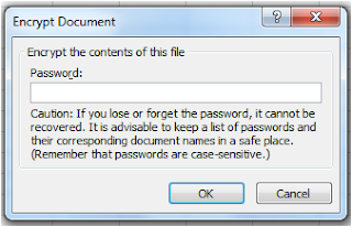
In order to use the encryption click the Microsoft Office Symbol, hover over the word Prepare and the Prepare menu will show. Click the Encrypt Document selection. Once you do this a dialog box will appear. Enter the password that you have selected.

Remember: do not forget the password or you will not be able to access your information.
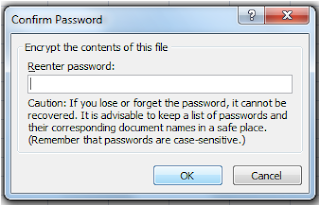
After you enter your password click the OK button. Once you have done this another dialog box will open this will ask you to confirm your password.

Microsoft put this in as a measure to ensure that you have input the password correctly. If the two passwords do not match you will get a dialog box that states Confirmation password is not identical.

The passwords must be put in the same. If you used a combination of uppercase and lowercase it must be the same. As an example, PassWord must be PassWord in order to work. If you typed PassWord and then Password you will get the confirmation error dialog box again. It is the same if you use alpha numeric passwords.

Hint: Keep in mind that there is no way that Excel can be set to force the user to save the Workbook with encryption.


Remember: Even Microsoft says that there is no way to retrieve a forgotten password, so if you forget the password you will have to reconstruct the Workbook.

If you want to make sure that the Workbook has been encrypted you can check by going to the Prepare selection again. If the Workbook has been encrypted there will be an orange/gold color around the icon as shown in the example above.

You can also check other workbooks in the same way.

Remember: Even Microsoft says that there is no way to retrieve a forgotten password, so if you forget the password you will have to reconstruct the Workbook.

The Document Inspector in Excel 07

Document Inspector

You can inspect your document to see what kind of information is associated with your Workbook.

1. Comments and Annotations
     a. If you have used any collaboration tools (we will talk about these later) it will check for this        information. Such as Comments, Track Changes.
2. Document Properties and
Personal Information a. Document properties also known as Metadata (Data about data. Such as the Author of the document, the date that the document was created, and the location on a computer or network that the document was created).
3. Custom XML Data
     a. XML (Extensible Markup Language, a form of code that the newer versions of Microsoft Office use that is Human readable and Machine readable. It serves to decrease the file size and reduce the possibility of corruption of the newer files that are created.) There are some portions of this that the file does not really need for the operation of the file and it can be removed without degrading the file in any way.
4. Headers and Footers
     a. Information saved in the Header and Footer Sections you can remove here.
5. Hidden Rows and Columns
     a. If you have hidden Rows or Columns that no one should see if you are sharing the information in this Workbook this will remove these hidden items.
6. Hidden Worksheets
     a. Much like the hidden rows and columns, although this will delete hidden Worksheets.
7. Invisible Content
     a. These are invisible object that you may have; no one can see them because they have been formatted to be invisible. This will remove them for you if you want.

After you have run the inspection you will get a second dialog box that appears. This will give you the opportunity to decide if you want to remove certain sections. As seen in the photo below. You will have a Remove All button next to the sections that have found information in them.

Once you click the remove all you can also Reinspect the document by clicking Reinspect, or you can close the dialog box.

Hint: 

Remember to save this workbook under another name otherwise you will lose all the information that you removed from your original Workbook. Then the only way to retrieve that information after it has been removed is to re-enter it in the Workbook.

The Prepare Choices in Excel 07

Properties: 

As shown in the picture below, under Document Properties, this dialog box shows;
1. The Author (typically the name that was put in at the installation of Microsoft Office.
2. Title (here you can enter a title for the document).
3. Subject (here you can enter a subject matter).
4. Keywords (here you can add keywords to help if you need to search for the file and cannot remember where you saved it, or the name of the file).
5. Category (here you can add a category name).
6. Status (here you can add a status to the Workbook, Complete, In Progress, or whatever you desire).
7. Comments (Here you can add comments).

After all the information is in simply click the X on the tan bar to close the dialog box.

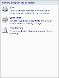
Print Using the Microsoft Symbol Button in Excel 07

Print

Print: Will open a dialog box that you can choose the printer that you want to use. All or specific pages that you want to print. Print Selection, Active Sheets, Entire Workbook, Ignore Print Areas, or Table. The Number of Copies you want.

Quick Print

Quick Print: Will send the information directly to the primary printer.

Print Preview

Print Preview: Will allow you to see what the Spreadsheets will look like when printed so you can make adjustments without using paper

Save and Save As in Excel 07

Save

Save and Save as will act the same the first time that you save a brand new workbook. After that the Save button will overwrite the existing document without asking if you wish to do so.

Save As

Will allow you to save a copy of the workbook anywhere you want to on your hard drive or network.
Excel Workbook: saves the workbook in Microsoft Office 07 format. No previous version of Office can open this without downloading a patch.
Excel Macro Enabled Workbook: saves a Macro Enabled workbook in Microsoft Office 07 format. We will discuss what Macros are later.
Excel Binary Workbook:
Excel 97-2003 Workbook: saves a copy of the workbook in a format that Microsoft Office 97 to 03 can open. This is a good format if you have friends that do not have Microsoft Office 07.
The Adobe PDF choice is on my system because I also have Adobe CS4 installed.
OpenDocument Spreadsheet: saves a file that can be opened with Open Office, this is a freeware version of Office and can be downloaded at http://www.openoffice.org/ .
PDF or XPS: will allow you to save as an Adobe PDF file or an XPS file. The PDF file is more commonly used for downloads on the internet as they are smaller in size than an Office file. They also have the distinction of being a read only file so it is harder for people to modify this type of document. You may have to download the patch for this if you have not used this option yet. Of you click on this option it will automatically determine if you have used it before or if the patch has been installed. If the patch has not been installed it will send you to the download site. Save the patch to your computer and install it, and now you are ready to publish this type of file.

Hint: If you want to modify the file in the future remember to save it as an Office Document as well. If you do not then you will have to recreate this document.

A Closer Look at the Menu Items New

New

Left Column

As you can see there are three main parts to the dialog box that appears after you press New. The left side gives you several choices that you can choose from. This has two headings in the column, Templates and Microsoft Online.
Under the Templates heading there are 4 choices
1. Blank and Recent
2. Installed Templates
3. My Templates…
4. New From Existing…
Under the Microsoft Office Online Heading there are 30 categories, each has more options listed.
1. Featured
a. Will vary depending on what templates are being featured at the time.
2. Access Databases
a. May be blank.
3. Agendas
a. Will show Icon views of Agenda Templates.
4. Books
a. Academic Books (show as a hyperlink in the center column)
i. When pressed it will show Icons for the templates you can choose.
b. Address and Phone Books (show as a hyperlink in the center column)
i. When pressed it will show Icons for the templates you can choose.
5. Brochures and Booklets
a. Brochures (Will show as a hyperlink in the center column)
i. When pressed it will show Icons for the templates you can choose.
6. Budgets
a. Business Budgets (Will show as a hyperlink in the center column)
i. When pressed it will show Icons for the templates you can choose.
b. Forecasts (Will show as a hyperlink in the center column)
i. When pressed it will show Icons for the templates you can choose.
c. Home Budgets (Will show as a hyperlink in the center column)
i. When pressed it will show Icons for the templates you can choose.
7. Calendars (These hyperlinks may change as to the years involved.)
a. 2012 Calendars (Will show as a hyperlink in the center column)
Excel 2007 by Shawn Ritter 2 Copyright 2012
i. When pressed it will show Icons for the templates you can choose.
b. 2011 Calendars (Will show as a hyperlink in the center column)
i. When pressed it will show Icons for the templates you can choose.
c. 2010 Calendars (Will show as a hyperlink in the center column)
i. When pressed it will show Icons for the templates you can choose.
d. Academic Year Calendars (Will show as a hyperlink in the center column)
i. When pressed it will show Icons for the templates you can choose.
e. Multiple-Year Calendars (Will show as a hyperlink in the center column)
i. When pressed it will show Icons for the templates you can choose.
f. Previous Year Calendars (Will show as a hyperlink in the center column)
i. When pressed it will show Icons for the templates you can choose.
g. Other Calendars (Will show as a hyperlink in the center column)
i. When pressed it will show Icons for the templates you can choose.
8. Cards
a. Identification Cards (Will show as a hyperlink in the center column)
i. When pressed it will show Icons for the templates you can choose.
b. Name and Place Cards (Will Show as a hyperlink in the center column)
i. When pressed it will show Icons for the templates you can choose.
c. Note Cards (Will Show as a hyperlink in the center column)
i. When pressed it will show Icons for the templates you can choose.
9. Charts and Diagrams
a. Business Charts (Will show as a hyperlink in the center column)
i. When pressed it will show Icons for the templates you can choose .
b. Floor plans and seating charts Will show as a hyperlink in the center column)
i. When pressed it will show Icons for the templates you can choose
c. Process Diagrams (Will show as a hyperlink in the center column)
i. When pressed it will show Icons for the templates you can choose
d. Smart Art Graphics (Will show as a hyperlink in the center column)
i. When pressed it will show Icons for the templates you can choose
e. Other Diagrams (Will show as a hyperlink in the center column)
i. When pressed it will show Icons for the templates you can choose
10. Faxes
a. Will show Faxes templates
11. Flyers
a. Real Estate Flyers (Will show as a hyperlink in the center column)
i. When pressed it will show Icons for the templates you can choose
b. Posters (Will show as a hyperlink in the center column)
i. When pressed it will show Icons for the templates you can choose
c. Signs (Will show as a hyperlink in the center column)
i. When pressed it will show Icons for the templates you can choose
12. Forms
a. Academic Forms (Will show as a hyperlink in the center column)
Excel 2007 by Shawn Ritter 3 Copyright 2012
i. When pressed it will show Icons for the templates you can choose
b. Applications (Will show as a hyperlink in the center column)
i. When pressed it will show Icons for the templates you can choose
c. Business Forms (Will show as a hyperlink in the center column)
i. When pressed it will show Icons for the templates you can choose
d. Community Forms (Will show as a hyperlink in the center column)
i. When pressed it will show Icons for the templates you can choose
e. Employment Forms (Will show as a hyperlink in the center column)
i. When pressed it will show Icons for the templates you can choose
f. Evaluations (Will show as a hyperlink in the center column)
i. When pressed it will show Icons for the templates you can choose
g. Math and Science Tables (Will show as a hyperlink in the center column)
i. When pressed it will show Icons for the templates you can choose
h. Medical and Healthcare Forms (Will show as a hyperlink in the center column)
i. When pressed it will show Icons for the templates you can choose
i. Personal Forms (Will show as a hyperlink in the center column)
i. When pressed it will show Icons for the templates you can choose
j. Quizzes and Tests (Will show as a hyperlink in the center column)
i. When pressed it will show Icons for the templates you can choose
k. Scorecards (Will show as a hyperlink in the center column)
i. When pressed it will show Icons for the templates you can choose
l. Sign-in and Sign-up Sheets (Will show as a hyperlink in the center column)
i. When pressed it will show Icons for the templates you can choose
m. Sports Forms (Will show as a hyperlink in the center column)
i. When pressed it will show Icons for the templates you can choose
n. Surveys (Will show as a hyperlink in the center column)
i. When pressed it will show Icons for the templates you can choose
o. Tournament Brackets (Will show as a hyperlink in the center column)
i. When pressed it will show Icons for the templates you can choose
13. Inventories
a. Will Show Icons for Inventories
14. Invoices
a. Bids and Quotes (Will show as a hyperlink in the center column)
i. When pressed it will show Icons for the templates you can choose
b. Estimates (Will show as a hyperlink in the center column)
i. When pressed it will show Icons for the templates you can choose
c. Finance Charges (Will show as a hyperlink in the center column)
i. When pressed it will show Icons for the templates you can choose
d. Packing Slips (Will show as a hyperlink in the center column)
i. When pressed it will show Icons for the templates you can choose
e. Purchase and Sales Orders (Will show as a hyperlink in the center column)
i. When pressed it will show Icons for the templates you can choose
Excel 2007 by Shawn Ritter 4 Copyright 2012
f. Sales Invoices (Will show as a hyperlink in the center column)
i. When pressed it will show Icons for the templates you can choose
g. Service Invoices (Will show as a hyperlink in the center column)
i. When pressed it will show Icons for the templates you can choose
h. Work Orders (Will show as a hyperlink in the center column)
i. When pressed it will show Icons for the templates you can choose
15. Labels
a. Mailing and Shipping Labels (Will show as a hyperlink in the center column)
i. Business Mailing Labels (Will show as a hyperlink in the center column)
1. When pressed it will show Icons for the templates you can choose
ii. Home Mailing Labels (Will show as a hyperlink in the center column)
1. When pressed it will show Icons for the templates you can choose
b. Office Labels (Will show as a hyperlink in the center column)
i. When pressed it will show Icons for the templates you can choose
c. Other Labels
16. Letterhead
17. Letters
a. Emails (Will show as a hyperlink in the center column)
i. When pressed it will show Icons for the templates you can choose
18. Lists and to-do Checklists
a. Academic Lists (Will show as a hyperlink in the center column)
i. When pressed it will show Icons for the templates you can choose
b. Business Lists (Will show as a hyperlink in the center column)
i. When pressed it will show Icons for the templates you can choose
c. Community Lists (Will show as a hyperlink in the center column)
i. When pressed it will show Icons for the templates you can choose
d. Home Lists (Will show as a hyperlink in the center column)
i. When pressed it will show Icons for the templates you can choose
e. Menus (Will show as a hyperlink in the center column)
i. When pressed it will show Icons for the templates you can choose
f. Trackers (Will show as a hyperlink in the center column)
i. When pressed it will show Icons for the templates you can choose
19. Memos
a. Will show Icons form Memos in the center column
20. Planners
a. Will Sow Icons for Planners in the center column
21. Plans and Proposals
a. Academic Plans (Will show as a hyperlink in the center column)
i. When pressed it will show Icons for the templates you can choose
b. Business Plans (Will show as a hyperlink in the center column)
i. When pressed it will show Icons for the templates you can choose
c. Bylaws, Policies, and Rules (Will show as a hyperlink in the center column)
Excel 2007 by Shawn Ritter 5 Copyright 2012
i. When pressed it will show Icons for the templates you can choose
d. Home Plans (Will show as a hyperlink in the center column)
i. When pressed it will show Icons for the templates you can choose
e. Instructions (Will show as a hyperlink in the center column)
i. When pressed it will show Icons for the templates you can choose
f. Medical and Healthcare Plans (Will show as a hyperlink in the center column)
i. When pressed it will show Icons for the templates you can choose
22. PowerPoint Presentations and Slides
a. Business Presentations (Will show as a hyperlink in the center column)
i. When pressed it will show Icons for the templates you can choose
23. Projects
a. Other Projects (Will show as a hyperlink in the center column)
i. When pressed it will show Icons for the templates you can choose
b. Project Calculators (Will show as a hyperlink in the center column)
i. When pressed it will show Icons for the templates you can choose
c. Games(Will show as a hyperlink in the center column)
i. When pressed it will show Icons for the templates you can choose
d. Office 2007 Document Themes (Will show as a hyperlink in the center column)
i. When pressed it will show Icons for the templates you can choose
24. Receipts
a. Will show Icons for Receipts in the center Column
25. Records
a. Academic Records (Will show as a hyperlink in the center column)
i. When pressed it will show Icons for the templates you can choose
b. Financial Records (Will show as a hyperlink in the center column)
i. When pressed it will show Icons for the templates you can choose
c. Home Records (Will show as a hyperlink in the center column)
i. When pressed it will show Icons for the templates you can choose
d. Human Resources Records (Will show as a hyperlink in the center column)
i. When pressed it will show Icons for the templates you can choose
e. Journals (Will show as a hyperlink in the center column)
i. When pressed it will show Icons for the templates you can choose
f. Ledgers (Will show as a hyperlink in the center column)
i. When pressed it will show Icons for the templates you can choose
g. Logs (Will show as a hyperlink in the center column)
i. When pressed it will show Icons for the templates you can choose
h. Medical and Other healthcare Records (Will show as a hyperlink in the center column)
i. When pressed it will show Icons for the templates you can choose
i. Other Records (Will show as a hyperlink in the center column)
i. When pressed it will show Icons for the templates you can choose
26. Reports
a. Analysis Worksheets (Will show as a hyperlink in the center column)
Excel 2007 by Shawn Ritter 6 Copyright 2012
i. When pressed it will show Icons for the templates you can choose
b. Expense reports (Will show as a hyperlink in the center column)
i. When pressed it will show Icons for the templates you can choose
c. Financial Reports (Will show as a hyperlink in the center column)
i. When pressed it will show Icons for the templates you can choose
d. Project and Status Reports (Will show as a hyperlink in the center column)
i. When pressed it will show Icons for the templates you can choose
e. Other Reports (Will show as a hyperlink in the center column)
i. When pressed it will show Icons for the templates you can choose
27. Schedules
a. Academic Schedules (Will show as a hyperlink in the center column)
i. When pressed it will show Icons for the templates you can choose
b. Business Schedules (Will show as a hyperlink in the center column)
i. When pressed it will show Icons for the templates you can choose
c. Itineraries (Will show as a hyperlink in the center column)
i. When pressed it will show Icons for the templates you can choose
d. Timelines (Will show as a hyperlink in the center column)
i. When pressed it will show Icons for the templates you can choose
e. Other Schedules (Will show as a hyperlink in the center column)
i. When pressed it will show Icons for the templates you can choose
28. Statements
a. Will show Icons for Statements in the center Column
29. Stationary and Specialty Paper
a. Handwriting Practice Paper (Will show as a hyperlink in the center column)
i. When pressed it will show Icons for the templates you can choose
b. Lined and Grid Paper (Will show as a hyperlink in the center column)
i. When pressed it will show Icons for the templates you can choose
c. Music Paper (Will show as a hyperlink in the center column)
i. When pressed it will show Icons for the templates you can choose
d. Other Specialty Paper (Will show as a hyperlink in the center column)
i. When pressed it will show Icons for the templates you can choose
30. Time Sheets
a. Will show Icons for Time Sheets in the center column

The Middle Column

1. Has a search option
2. Has an Icon option

The Third Column / Right Side

 Shows a brief preview of the document