The Quick Access Toolbar in Excel 07

The Quick Access Toolbar is located to the right of the Microsoft Office Symbol and Above the Home Tab.
Right out of the box, initial install, there are three buttons by default; Save, Undo, and Redo. If you want to you can add buttons or remove buttons from the Quick Access Tool Bar. There are a few of ways that we can do this.

The Quick Access Toolbar Button

     To the right of the Quick Access Toolbar there is a symbol that looks like a line above a triangle that is pointing down, this is actually a button.
   
     When you press the button a dialog box appears. With this dialog box you can add or remove buttons from a standard list. As you can see there are some that have a check-mark to the left of them. These are the buttons that will show in the Quick Access Toolbar.

     To add more buttons just click on the word, for instance New, This will add the New Spreadsheet Button to the Quick Access Toolbar; the Dialog Box will close after you click. If you want to add more of the predefined buttons then you can repeat the same steps as often as you want.

     To remove the button from the list, simply click on the name of the button that you wish to remove from the Quick Access Toolbar and the check-mark will be removed, the Dialog Box will close, and it will remove the button from the Quick Access Toolbar.

     There are three other buttons on the Customize Quick Access Toolbar; they are More Commands, Show Below the Ribbon, and Minimize the Ribbon.

More Commands

     The More Commands Button will open another Dialog Box; this dialog box has many options for
customizing Microsoft Excel. I will talk about most of them later on in the book. For now I will discuss
the Customize the Quick Access Toolbar, in the Customize Section.

     This Dialog Box is split into many parts; On the right side we have a list of sections that we can
access, there is the Choose commands from drop down, below that we have the command buttons for
that particular command group. Below that we have the Show Quick Access Button Below the Ribbon
check box. Next we have the Add and Remove Buttons. Then the Customize Quick Access Toolbar drop
down, here we can choose if we want to apply the changes in the Quick Access Toolbar to all Documents
or just this particular Spreadsheet. Below that we have a list of the buttons that will appear in the Quick
Access Toolbar. Then we have the Reset Button which will reset the Quick Access Toolbar to the default
settings. The Modify Button applies to special buttons that you can create for Macros, we will talk about
these later. To the right of the button list there are two buttons that we can use to change the order of
the buttons on the Quick Access Toolbar, the closer the button is to the top of the list the closer to the
Office Symbol it will be. We then have the OK and Cancel buttons. If we made changes to the list we
need to click the OK button for those changes to take effect, if we use the Cancel button it will not keep
the changes that we have just made.

Add a Quick Access Button from a Group

     There is another way to add a button to the Quick Access Toolbar using the right mouse button.
If you want to add the Insert Picture Button, go to the Insert Tab, right mouse click on the Picture Icon
and click the Add to Quick Access Toolbar.

Show Below the Ribbon

     The Show Below the Ribbon, option will move the Quick Access Toolbar from the default location to bellow the ribbon.  When you do not know that this is a feature and someone has moved the Quick Access Toolbar it is hard to find. I know because before I realized that this was an option it happened to me.
When the Quick Access Toolbar is below the Ribbon the choice changes to Show Above the Ribbon.

Minimize the Ribbon

     The Minimize the Ribbon is another option that Microsoft has given. When you use this option
the Workbook area becomes larger. This is an option that Microsoft did not advertize. I learned about
this option when I was told that I was going to be sowing others how to use Microsoft Office 2007.
There was no training that neither I nor my boss received.

     The program was installed on one computer in my classroom; someone had accidentally removed the Ribbon before either of us had seen the new program. It took awhile but my boss figured it out and informed me as to how to fix it.

     To Minimize the Ribbon with the control button, click the Button and then click on the last choice, Minimize the Ribbon. See the picture to the right. With the Ribbon Minimized to see the groups on the ribbon just click on the tab name such as Home, Insert, Page Layout, etc…

     To maximize the Ribbon you can click on the Quick Access Toolbar Button again and uncheck the Minimize the Ribbon. This will restore the Ribbon to its original state.

The Quick Access Toolbar Right Mouse Click 

     With a quick click or the Right Mouse Button you can remove a button from the Quick Access Toolbar, all you have to do is Right Mouse Click the Icon and use the Remove from Quick Access Toolbar.

The Alt Key

NOTE: You can use either lower case or upper case letters. It may take a bit longer but it works.

If for some reason your mouse dies these is still a way that you can navigate the Excel Workbook. That way is the Keyboard. By pressing the ALT Key Numbers and Letters appear. By pushing the corresponding key you can Navigate

1. F – will open the Office Symbol Dialog Box
2. 1 – The First Button on the Quick Access Tool Bar
3. 2 – The Second Button on the Quick Access Tool Bar
4. 3 – The Third Button on the Quick Access Tool Bar
5. H – will display the Home Tab
6. N – will display the Insert Tab
7. P – will display the Page Layout Tab
8. M – will display the Formulas Tab
9. A – will display the Data Tab
10. R – will display the Review Tab
11. W – will display the View Tab
12. L – will display the Developer Tab
F will open the Office Symbol Dialog Box

Once the F or Office Symbol Dialog box opens there will be other choices. After you make a single choice the Dialog will close. If you want to do something else you will need to go through the motions again.

1. N – will open a New Spreadsheet
2. O – will open the Open Dialog Box
3. S – will Save the Workbook
4. A – will open the Save As Dialog Box
5. F – will open up the Save As Choices
6. P – will open the Print Dialog Box
7. W – will open the Print Choices
8. E – will open the Prepare Choices
9. D – will open the Send Choices
10. U – will open the Publish Choices
11. C – will Close the Spreadsheet
12. I – will display the Excel Options Dialog Box
13. X – will Exit the Excel Program

1  –  The First Button on the Quick Access Tool Bar. If the Save Button is the first button, by default on install, then the number 1 will Save the Workbook.
2 – The Second Button on the Quick Access Tool Bar.  If the Undo Button is the first button, by default on install, then the number 2 will Undo the last modification made to the Workbook.
3 –  The Third Button on the Quick Access Tool Bar,  If the Redo Button is the first button, by default on install, then the number 3 will Redo the last Undo made to the Workbook.

H will display the Home Tab

There are two ways to Navigate the Submenus, to Navigate you can either press the letter associated with the ALT Tab or you can use your Arrow Keys. If you are in one of the Menus the ESCAPE Key will go back one level.

The Clipboard Group

1. V will bring up the Paste Menu
     a. P – for Paste
     b. F – for Formulas
     c. V – for Paste Values
     d. B – for No Borders
     e. T – for Transpose
     f. N – for Paste Ink
     g. S – for Paste Special
     h. H –for Paste as Hyperlink
     i. A – for As Picture
          i. C – for Copy as Picture
          ii. U – for Past as Picture
          iii. I – (the capital i) for Paste Picture Link
2. X – to Cut a selected area
3. C – to Copy a selected area
4. FP – to copy the Format from a selected area
5. FO – will bring up the Clipboard Dialog

The Font Group

6. FF – will open the Font Face Dialog
7. FS – will open the Font Size Dialog
8. FG – is the command to take the Font Size up one size
9. FK – is the command to reduce the Font Size one size
10. 1 – will Bold the selected area
11. 2 – (The number 2) will Italicize the selected area
12. 3 – (The Number 3) will Underline the selected area
13. B – will add Borders to the selected area
14. H – will bring up the Cell Background Color Dialog
15. FC – will bring up the Font Color Dialog
16. FN – will Bring up the Format Cells Dialog Box – Font Tab

The Alignment Group

17. AT – Top Align
18. AM – Middle Align
19. AB – Bottom Align
20. FQ – Orientation, or test angle
21. W – Wrap Text
22. AL – Align Left
23. AC – Align Center
24. AR – Align Right
25. 5 – Decrease Indent
26. 6 – Increase Indent
27. M – Merge and Center
28. FA – will bring up the Format Alignment Dialog Box – Alignment Tab

Number Group

29. N – will bring up the Number Dialog Box
30. AN – will bring up the (Accounting Number Format) Currency Dialog Box
31. P –Percent Style
32. K – Comma Style
33. 0 (Zero, the number not the letter) – Decrease Decimal
34. 9 – Increase Decimal
35. FM - will bring up the Format Number Dialog Box – Number Tab

The Style Group

36. L – Opens the Conditional Formatting Dialog Box
37. T – Opens the Format as Table Dialog Box
38. J – Opens the Styles Dialog

The Cells Group

39. I – Opens the Insert Dialog Box
40. D – Opens the Delete Dialog Box
41. O (ooh, the letter not the number) – Opens the Format Dialog Box

The Editing Group

42. U – Opens the AutoSum Dialog Box
43. FI (I capitol i) – Opens the Fill Dialog Box
44. E – Opens the Clear Dialog Box\
45. S –Opens the Sort & Filter Dialog Box
46. FD –Opens the Find & Select Dialog Box

You can do the same for all the Tabs and Groups within Excel.

Navigating a Spreadsheet Part 1

Remember: The size of the Scroll Bars will vary with the amount of information held Within the Workbook.

Navigating a Spreadsheet,

There are several ways in which to Navigate a Spreadsheet.

The Scroll Bars

1. Vertical Scroll Bar, this allows us to move up and down the Spreadsheet. It is located
at the right hand side of the Workbook Window.

2. On the Vertical Scroll Bar there are two Arrows, one on top and the other on the
bottom. You can use these to Scroll Up and Down The Top Arrow will move the
Spreadsheet towards the Top or Row 1, the Bottom Arrow will move the Spreadsheet
towards the bottom or towards row 1048576.

3. The Horizontal Scroll Bar, This is located at the bottom of the Workbook just above the
Status bar and to the right of the Tabs.

4. The Horizontal Scroll Bar has two arrows at either side of it. The one to the left will
scroll back towards Column A, the one on the right will scroll towards Column XSD (the
last Column in the Spreadsheet)

The Mouse Wheel

1. If you have a Wheel Mouse you can push down on the wheel you will get a Four Pointed arrow, this will allow you to move any direction on the Spreadsheet that you >want. One thing about this that I have discovered is that if you want to scroll down quickly, before you click the wheel, get close to the top of the Spreadsheet Cells. Then after you click the wheel the closer you get to the bottom of the Spreadsheet the faster it will scroll down.
The wheel also moves you up and down the Workbook, if you roll the wheel forward it will take you towards the top of the Spreadsheet, Row 1. If you roll the wheel backwards it will move the Spreadsheet down, towards Row 1048576.

The Mouse Left Button

1. Take your Mouse and hover over any Cell then click the Left Mouse Button and it will put you into that cell

The Tab Key

1. The Tab Key will take you one Cell to the right
2. SHIFT + Tab will take you one Cell to the left

The Enter Key

1. The ENTER Key will take you one Row down
2. SHIFT + ENTER will take you one Row up

The Address Bar

1. Will take you to the Cell Address that you tell it to
     a. Once you enter the Cell Address hit Enter

The Arrow Keys

1. Up Arrow will take you one Cell up
2. Down Arrow will take you one Cell Down
3. Left Arrow will take you one Cell to the Left
4. Right Arrow will take you one Cell to the Right

CTRL + Arrow Keys (Assuming you are starting from Cell A1 with information to cell H35)

1. First use of CTRL + Down Arrow will move you to Cell A35
2. Second use of CTRL + Down Arrow will move you to Cell A 1048576
3. Firs t Use of CTRL + Up will move you to Cell A35
4. Second use of Up Arrow will move you to Cell A1
5. First use of CTRL + Right Arrow will move you to H1
6. Second Use of CTRL + Right Arrow will move you to Cell XFD
7. First use of CTRL + Left will move you to Cell H1
8. Second use of CTRL + Left Arrow will move you to Cell A1

CTRL + Arrow Keys (Assuming you are starting from Cell A1 with information to cell H35 with missing information in Cell A14 and missing information in Cell E1)

1. First use of CTRL + Down Arrow will move you to Cell A13
2. Second use of CTRL + Down Arrow will move you to Cell A15
3. Third use of CTRL + Down Arrow will move you to Cell A35
4. Fourth use of CTRL + Down Arrow will move you to Cell A 1048576
5. Firs t Use of CTRL + Up will move you to Cell A35
6. Second use of Up Arrow will move you to Cell A15
7. Third Use of CTRL + Up will move you to Cell A13
8. Second use of Up Arrow will move you to Cell A1
9. First use of CTRL + Right Arrow will move you to D1
10. Second Use of CTRL + Right Arrow will move you to Cell F1
11. Third use of CTRL + Right Arrow will move you to H1
12. Fourth Use of CTRL + Right Arrow will move you to Cell XFD
13. First use of CTRL + Left will move you to Cell H1
14. Second use of CTRL + Left Arrow will move you to Cell F1
15. Third use of CTRL + Left will move you to Cell D1
16. Fourth use of CTRL + Left Arrow will move you to Cell A1

Go To

With the Go To you can navigate to any Cell in the Spreadsheet that you want to, similar to the Address Bar. The quick way to get to Go To is CTRL + G.

The fx is a Button and Functions Dialog Bar

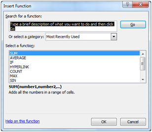
     The fx is not only there to tell you that the Function Dialog bar is coming up next, it is actually a button. Once you press this symbol you will get a dialog box that gives you several choices of prebuilt functions that Excel has. I will talk more at length about these later. I will also explain the parts of the dialog box later.

     There are also a few more ways that we are able to access the Functions Dialog box, using the Auto-sum button or it can be accessed from the Formulas Tab. I will go into depth about these choices later.

     The Function Dialog Bar shows the function as opposed to the total that is shown by default in the Workbook Cell. As we see here in cell A4 we see 3200, yet in the Functions Dialog Bar we see =SUM(A2:A3) or the actual Function its self.










    If the Function is longer than the functions dialog box the code for the function will wrap around much the same as a paragraph in Microsoft Word. Two arrows will appear at the right side of the screen just to the left of the double chevron. If you use the single arrows you can scroll up or down one line at a time. If you use the double chevron it will expand the Functions Dialog Bar and show several lines.





Normal Function Dialog View


Expanded Function Dialog View

      The position of the arrows will change slightly from the collapsed view of the Functions Dialog Box, instead of being beside each other as in the previous example. In the expanded view the buttons are stacked.

One Important Note about Excel

     Working with Excel will become easier once you realist that EXCEL DOES NOT CARE ABOUT YOU. Excel is considered the SNOB of the Microsoft Office Suite. The only things that Excel cares about are numbers, and numbers are the only thing. Not you, not text, or labels as Microsoft calls them. Not even other Excel Workbooks.


     Excel has been set up to automatically by default have text to the left of the Cell and numbers to the right of   the Cell.

The Quick Access Toolbar

The Quick Access Toolbar is located to the right of the Microsoft Office Symbol and Above the Home Tab.
Right out of the box, initial install, there are three buttons by default; Save, Undo, and Redo. If you want to you can add buttons or remove buttons from the Quick Access Tool Bar. There are a few of ways that we can do this.

The Quick Access Toolbar Button

To the right of the Quick Access Toolbar there is a symbol that looks like a line above a triangle that is pointing down, this is actually a button.

When you press the button a dialog box appears. With this dialog box you can add or remove buttons from a standard list. As you can see there are some that have a checkmark to the left of them. These are the buttons that will show in the Quick Access Toolbar.

To add more buttons just click on the word, for instance New, This will add the New Spreadsheet Button to the Quick Access Toolbar; the Dialog Box will close after you click. If you want to add more of the predefined buttons then you can repeat the same steps as often as you want.

To remove the button from the list, simply click on the name of the button that you wish to remove from the Quick Access Toolbar and the checkmark will be removed, the Dialog Box will close, and it will remove the button from the Quick Access Toolbar.

There are three other buttons on the Customize Quick Access Toolbar; they are More Commands, Show Below the Ribbon, and Minimize the Ribbon.

More Commands

The More Commands Button will open another Dialog Box; this dialog box has many options for customizing Microsoft Excel. I will talk about most of them later on in the book. For now I will discuss the Customize the Quick Access Toolbar, in the Customize Section.

This Dialog Box is split into many parts; On the right side we have a list of sections that we can access, there is the Choose commands from drop down, below that we have the command buttons for that particular command group. Below that we have the Show Quick Access Button Below the Ribbon check box. Next we have the Add and Remove Buttons. Then the Customize Quick Access Toolbar drop down, here we can choose if we want to apply the changes in the Quick Access Toolbar to all Documents or just this particular Spreadsheet. Below that we have a list of the buttons that will appear in the Quick Access Toolbar. Then we have the Reset Button which will reset the Quick Access Toolbar to the default settings. The Modify Button applies to special buttons that you can create for Macros, we will talk about these later. To the right of the button list there are two buttons that we can use to change the order of the buttons on the Quick Access Toolbar, the closer the button is to the top of the list the closer to the Office Symbol it will be. We then have the OK and Cancel buttons. If we made changes to the list we need to click the OK button for those changes to take effect, if we use the Cancel button it will not keep the changes that we have just made.

Add a Quick Access Button from a Group

There is another way to add a button to the Quick Access Toolbar using the right mouse button. If you want to add the Insert Picture Button, go to the Insert Tab, right mouse click on the Picture Icon and click the Add to Quick Access Toolbar.

Run Compatibility Checker

The Compatibility Checker will check to see if Microsoft Office 2007 features will be compatible with earlier versions of Microsoft Office.  In the case that they are not the program will convert the non compatible items into pictures so the older versions of Microsoft Office will display them.  In this picture there were no compatibility problems

The times that this is most important are when the Workbook has been opened from a previous version and is going to be saved again in that same version.  If the Workbook is opened in Microsoft Office 2007 the options will still be editable but if opened in a previous version they will not be able to be edited.

For the most part the compatibility checker will check for newer items such as Smart Art and the newer Word Art.

The Mark as Final Option in Excel 2007

What does Mark as Final do for me?

Mark as Final will make your Workbook a Read Only, similar to the Digital Signature, however, the Digital Signature add another level of security.  The Mark as Final can be removed and then the information changed and then the Mark as Final can be added again.

In order to mark a workbook as final
     1. Click the Microsoft Office Symbol
     2. Hover over the Prepare option
     3. Click the Mark as Final option
     4. A Dialog Box will appear
     5. Click the OK Button
     6. Once you click the OK button a couple of things will happen.
          a. The Workbook will automatically save.
          b. Another Dialog Box will appear, the first time only unless you do not check the “Don’t show this message again” check box.
          c. An Icon will appear in the Status Bar.
          d. The Groups will become grayed out. With the exception of a few options.
          e. The Title Bar will show the words Read Only.

Remember: if you cannot access the options in the groups that you want the Workbook is in the Mark as Final, or read only mode.

To Remove the Mark as Final or Read Only
     1. Click the Microsoft Office Symbol.
     2. Hover over the Prepare option
     3. Click the Mark as Final button; this will have an orange / gold square around it.
     a. After this is done all the buttons in the groups should be active again.