Link Excel 07 to PowerPoint 07

Things to keep in mind when linking a chart from excel into PowerPoint

1.       Save the excel workbook on the tab that the chart is on.  Otherwise it will not show the correct information.

2.       Unless you want to take the long way to copy and paste remember to check the Link checkbox.

Steps to linking the excel chart to PowerPoint

1.  Open the PowerPoint presentation that you wish to add the chart into.
2. Create a new blank slide.
3. On the blank Slide go to the Insert Tab and choose the Object button.
4. Make sure that you choose the Create From File choice.
5. Browse to the file location and choose the excel workbook you want.
6. Be sure to check the Link check box (otherwise you will have done the long way of copy paste).
7. Click OK.
8. Save the PowerPoint presentation and next time you open the presentation it will ask if you wish to update the link.  If you do click the Update Link button or if not click Cancel.

Excel Filtering 07

What does filtering do for me?

Filtering can help if you want to data mine, mine for information.  I can view my information by Males only and by SSG, or by Females and SSG. Anything that I want I can filter for as long as it is in my information.

Where to find the Filter Button?

You can find the Filter button on the Home Tab at the right hand side under Sort and Filter.

Set up Filtering

Click into your Labels row (Last Name, First Name, etc…)

Choose the Filter Button.

Drop Down arrows will appear in your Labels, in the lower right corner.

You can select what you wish to view by making sure that the check box has a check mark in it. The quickest way to uncheck everything is to click the (select all).

You may filter by as many criteria as you need.

Cautions when filtering

If you save the filtered workbook and open it again and you have not cleared the filters the information will still be filtered.  After the heart attack moment check to see

If the filter buttons are on

Are the Numbers to the left out of sequence and blue?

Is the filter button glowing orange/gold?

If the answer to any of these questions a yes, the filters are still turned on and the information is still filtered.

Excel Sorting

Things to be careful of when sorting

1.       If you choose the Column Header such a C, and then choose sort, you need to make sure that the choice Expand the Selection is selected or you will mix your record information up.

2.       If you click into an empty column and then try to sort nothing will happen.

3.       If you are outside of the range you will get an error message.

Normal Sorting

1.       Click into the information, a populated column, and click the sort button A to Z or Z to A depending on how you wish to sort.

a.        You can find the sort buttons on the Home Tab at the right hand side under Sort and Filter.

b.      Or you can find the Sort buttons on the Data Tab.

Custom Sorting Options

1.       Sort By: Gives a list of Column Headers that you can sort by.

2.       Sort On: Values, Cell Color, Font Color, Cell Icon.

a.       If you sort by Cell Color or Font Color you will need to create multiple sorts for the same column.  You can adjust the colors to fit how you wish them to be displayed.  Red then yellow then Green, Green then Red then Yellow.

3.       Order: A- Z, Z – A, Custom List

a.       Custom Lists will arrange the information in accordance to the specified list.  Sunday, Monday, Tuesday, Wednesday, Thursday, Friday, Saturday.

4.       My data has headers: Check box.

Custom Sorting

To sort by more than one field you need to choose Custom Sorting.  In combination with the above options you can sort various different ways.

1.       Click Add Level.

2.       Choose what column that you want to sort by.

3.       Choose what to sort on, Values being the most common.

4.       Choose how to sort, A – Z being the most common.

5.       Repeat as needed for as many criteria you wish to sort by.  (lather, rinse, repeat)

Excel Conditional formatting Office 07

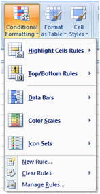
 Conditional formatting can be used to have Excel determine whether or not something falls within a specific guideline.  Say for instance that you want to track when someone needs retested, you could have the cell change color automatically depending on criteria.  The Conditional Formatting button is found on the Home Tab.  It has some prebuilt functionality, however if you need to you can create your own rules.

Conditional formatting for the example is as follows:

Notice the first line of the text is blue.  This has a conditional format associated with it that shows all the dates before 5/12/11 with a blue background.

              

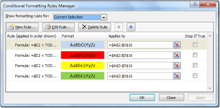
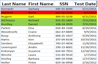
In order for us to show all of the information with the blue we need to be careful how we write the formula inside of the conditional formatting dialog.  Also, the placement of each rule is important here due to the fact that if I have the rules listed out of order the colors will be off.  For instance f I have the rule for 90 days out at the top all of the highlighted areas would be green not the rainbow as above.

If for some reason the formatting does not look correct on the Excel work sheet, when you have finished. It could be due to the fact that the Conditions are out of order, reopen the Conditional Formatting rules and make sure that the rule with the lowest value is at the top.  Another possibility is that the Cancel button was hit instead of the Apply or OK buttons.

If for some reason the Blue does not appear  open the Condition Formatting Rules and move the blue rule up by using the arrows.  These conditional formatting rules should be at the bottom of the list.  We can move them by using the arrows in the upper right hand section of the Condition Formatting Rules Manager, see below.

Using the Today Function

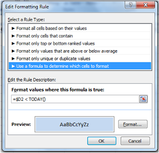
We will use the today function and compare it to cell D2 to get the required color.  In this case the formula would read; =$D2 < Today(). The next rule would be; =&D2 < Today()+30.  The third rule would be; =$D2 < Today()+60, and the last one is; =$D2 < Today()+90.

To conditionally format a single column of dates looking for 30, 60, and 90 days out.  Select the column header and go to the Conditional Formatting button, choose Manage Rules this will bring a dialog box up that we can use to create many different rules.  Click the New Rule button, another dialog box will appear.  Choose Format only cells that contain and fill in the information in the first dialog =Today() and the second dialog =Today()+30 this will select a date range for the next 30 days.  Format the cell fill color to red.

For the range of 60 days out we will want to make a second rule, click the New Rule button, another dialog box will appear.  Choose Format only cells that contain and fill in the information in the first dialog =Today()+31 and the second dialog =Today()+60 this will select a date range for the next 30 days.  Format the cell fill color to yellow.

For the range of 90 days out we will want to make a second rule, click the New Rule button, another dialog box will appear.  Choose Format only cells that contain and fill in the information in the first dialog =Today()+61 and the second dialog =Today()+90 this will select a date range for the next 30 days.  Format the cell fill color to green.

Alternating Cell Color

In order to create alternating row colors that will not move when sorted we can use conditional formatting.  These conditional formatting rules should be at the bottom of the list.  We can move them by using the arrows in the upper right hand section of the Condition Formatting Rules Manager, see below

If you wish to have alternating row colors, using conditional formatting, see image to the left.  We need to select the area that we wish to have the alternating lines of color.  I have chosen columns A to F and rows 1 to 19.

We need to go in to the conditional formatting Manage Rules and choose Use a formula to determine which cells to format.

In the Format values where this formula is true:, section we need to type in the following rule.

=mod(row(),2)=1

The =mod() means that we want to modify something, the selected area.

The row() or rows are what we are modifying.

The 2 tells Excel how many rows we are going to alternate the cell colors, see the example above.  Every two rows are colored.

The =1 tells Excel where to start the colorizing, in this case I started at row 1.  Our choices ore 0 (Zero) or 1, 0 starts at row 2 and 1 starts at row 1.

Excel Basic Formulas and Functions

Formulas and Functions have some things in common.  They both start with the EQUAL sign and have cell references, they both give results for the equation.  It depends on how you want to get there.  Sometimes Formulas are the only way when there is no function that can match your needs.

Basic Formulas

Formulas are considered the long hand version of Functions.  A formula for adding a column or a row would be:

Addition: =A1+A2+A3+A4+A5+A6…  As you can see the possibility of mistakes are very real, you may forget a cell reference or a plus sign, thereby breaking your equation. 

Subtraction: =A1-A2-A3…  Again, the possibilities of mistakes are great.

Mixed Addition and Subtraction: =A1-A2+A3…  There are two possible problems with this scenario, one if the person that you give this worksheet to does not know where to place the amount being subtracted then the results will not be what is expected.  Two the possibilities of mistakes are great.

Multiplication: =A1*A2*A3… Most of the time multiplication is done for only one or two cells this method works rather well.

Division: =A1/A2… most of the time division is done with only two cells this method works rather well.

Implied IF: =A1>A2…  Will give either a True or False value in word form.

Basic Functions

Functions are like the shorthand method of getting the desired results.  There are times when I need to use functions because there are no formulas that will work, mostly for the intermediate functions.

Addition: =SUM(A1:A6)… This gives the same results as the Addition Formula

Subtraction: =SUM(A1:A6)… Looks like the addition method, yes it is.  Here we are able to put a minus sign in front of the value in the cell and I now know exactly where the negative value is.

Multiplication: =PRODUCT(A1:16)… This will multiply everything in that range.

Division: =QUOTENIT(A1,A2)… This will only allow two cells to be used.  It is easier to us the formula in this case.

Today(): Pulls the date form the computer in a dynamic format.  If you save the document today it will have today’s date, however if you open the document tomorrow it will have tomorrows date instead.  This is a good function to use if you have conditional formatting and want to know the record that is within 30, 60, or 90 days.

Excel Cell References Absolute VS Relative

Absolute Value

Absolute Value: when a cell value remains the same no matter if it is copied and pasted, moved, or has been filled down or over.  An example of an Absolute Value $A$1 + $A$2 when copied to column B will show as $A$1 + $A$2

There are two ways to create an Absolute Value, One have the cursor by the value that you want to be the Absolute (either before the letter, between the letter and the number, or directly after the number of the field address) and use the F4 key on the function key row.  Two manually insert the $ symbol as you are typing the cell reference in. 

Relative Value

Relative Value: when the value of the starting cell changes from row to row or column to column.  An example of a Relative Value A1+A2, when copied to column B will show as B1 + B2

Why do we need to know about Cell References?

Suppose that you need to have a spreadsheet that has a single value that is used for many different calculations and that this value changes often,  If you do not wish to go into the formula and change it all the time and then remember to go into every formula and make the change, then the Absolute Cell Reference will assist us.

In the examples it may not be a problem to change every Formula, however, if we have 100 or 200 Formulas to change imagine how easy it may be to forget to change one or use the incorrect value.

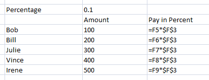
In these examples we see that there are two different results with the same information, one has Relative Cell Reference and the other has Absolute Cell Reference.

 Relative Reference

Absolute Reference

See where we get a VALUE error in the Relative reference sample that is caused by the formula attempting to calculate a number and text.  See Example of Relative Formula.  In the Absolute Reference we can see the formula has worked as expected, see Example Absolute Formula.

Relative Formula

 

Absolute Formula

See how in the Absolute Formula the Dollar signs locked the cell to F3.  Now I only have to change one value and everything else will recalculate by itself.

Hint

We can toggle between the Values and the Formulas / Functions by using CTRL+` (Normally the ` symbol is located above the TAB key).

Excel Fill Handle and Using Preexisting Lists

Fill Handle


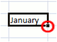
The fill handle is the little black square in the lower right hand corner of the selected cell. It can fill down Days of the week Months of the year and number sequences. We can also make custom lists that we can then fill down as well.

The examples to the right show the three steps to use the fill handle. First we type in what we want in our list and then hover over the fill handle, the curser will turn to a small black plus sign. Not the one with the arrows. Hold your left mouse button down and drag in the direction that you wish to have your list. A dotted border will encompass the area where you are dragging and a small text will appear to the side, once you let go of the fill handle it will place you list in the selected area. 

As you can see by the example to the right the list is automatically generated.  This works with Days of the week, abbreviated or spelled out, in all upper case, lower case or normal.  This works with numbers and number sequences you can count by ones two threes or whatever you need to.  With counting by two's, three's or other such types you need to set it up.  You will need to type the first number in a cell, then depending on the direction that you wish to see the information in the adjacent cell, below or to the left, enter your second number in the series.  Once this is done select both the cells that have your number in them and then use the fill handle to do the rest.

Excel Error Codes

#####	The numeric value is too wide to display within the cell. You can re-size the column by dragging the boundary line between the column headings.
#VALUE!	You entered a mathematical formula that references a text entry instead of a numerical entry.
#DIV/0!	You tried to divide a number by zero. This error often occurs when you create a formula that refers to a blank cell as a divisor.
#NAME?	You entered text in a formula that Excel doesn't recognize. You may have misspelled the name or function, or typed a deleted name. You also may have entered text in a formula without enclosing the text in double quotation marks.
#N/A	This error occurs when a value is not available to a function or a formula. If certain cells on your worksheet contain data that is not yet available, enter #N/A in those cells. Formulas that refer to those cells will then return #N/A instead of attempting to calculate a value.
#REF!	The #REF! error value occurs when a cell reference is not valid. You probably deleted a cell range that is referenced in a formula.
#NUM!	The #NUM! error value occurs when you use an invalid argument in a worksheet function.
#NULL!	You specified an intersection of two ranges in a formula that do not intersect.

Excel CTRL combination shortcut keys

Key	Description
ALT+=	Auto Sum
CTRL+SHIFT+(	Unhides any hidden rows within the selection.
CTRL+SHIFT+)	Unhides any hidden columns within the selection.
CTRL+SHIFT+&	Applies the outline border to the selected cells.
CTRL+SHIFT_	Removes the outline border from the selected cells.
CTRL+SHIFT+~	Applies the General number format.
CTRL+SHIFT+$	Applies the Currency format with two decimal places (negative numbers in parentheses).
CTRL+SHIFT+%	Applies the Percentage format with no decimal places.
CTRL+SHIFT+^	Applies the Exponential number format with two decimal places.
CTRL+SHIFT+#	Applies the Date format with the day, month, and year.
CTRL+SHIFT+@	Applies the Time format with the hour and minute, and AM or PM.
CTRL+SHIFT+!	Applies the Number format with two decimal places, thousands separator, and minus sign (-) for negative values.
CTRL+SHIFT+*	Selects the current region around the active cell (the data area enclosed by blank rows and blank columns). In a PivotTable, it selects the entire PivotTable report.
CTRL+SHIFT+:	Enters the current time.
CTRL+SHIFT+"	Copies the value from the cell above the active cell into the cell or the Formula Bar.
CTRL+SHIFT+Plus (+)	Displays the Insert dialog box to insert blank cells.
CTRL+Minus (-)	Displays the Delete dialog box to delete the selected cells.
CTRL+;	Enters the current date.
CTRL+`	Alternates between displaying cell values and displaying formulas in the worksheet.
CTRL+'	Copies a formula from the cell above the active cell into the cell or the Formula Bar.
CTRL+1	Displays the Format Cells dialog box.
CTRL+2	Applies or removes bold formatting.
CTRL+3	Applies or removes italic formatting.
CTRL+4	Applies or removes underlining.
CTRL+5	Applies or removes strikethrough.
CTRL+6	Alternates between hiding objects, displaying objects, and displaying placeholders for objects.
CTRL+8	Displays or hides the outline symbols.
CTRL+9	Hides the selected rows.
CTRL+0	Hides the selected columns.
CTRL+A CTRL+A  cont…	Selects the entire worksheet. If the worksheet contains data, CTRL+A selects the current region. Pressing CTRL+A a second time selects the current region and its summary rows. Pressing CTRL+A a third time selects the entire worksheet. When the insertion point is to the right of a function name in a formula, displays the Function Arguments dialog box. CTRL+SHIFT+A inserts the argument names and parentheses when the insertion point is to the right of a function name in a formula.
CTRL+B	Applies or removes bold formatting.
CTRL+C	Copies the selected cells. CTRL+C followed by another CTRL+C displays the Clipboard.
CTRL+D	Uses the Fill Down command to copy the contents and format of the topmost cell of a selected range into the cells below.
CTRL+F	Displays the Find and Replace dialog box, with the Find tab selected. SHIFT+F5 also displays this tab, while SHIFT+F4 repeats the last Find action. CTRL+SHIFT+F opens the Format Cells dialog box with the Font tab selected.
CTRL+G	Displays the Go To dialog box.  F5 also displays this dialog box.
CTRL+H	Displays the Find and Replace dialog box, with the Replace tab selected.
CTRL+I	Applies or removes italic formatting.
CTRL+K	Displays the Insert Hyperlink dialog box for new hyperlinks or the Edit Hyperlink dialog box for selected existing hyperlinks.
CTRL+N	Creates a new, blank workbook.
CTRL+O	Displays the Open dialog box to open or find a file. CTRL+SHIFT+O selects all cells that contain comments.
CTRL+P	Displays the Print dialog box. CTRL+SHIFT+P opens the Format Cells dialog box with the Font tab selected.
CTRL+R	Uses the Fill Right command to copy the contents and format of the leftmost cell of a selected range into the cells to the right.
CTRL+S	Saves the active file with its current file name, location, and file format.
CTRL+T	Displays the Create Table dialog box.
CTRL+U	Applies or removes underlining. CTRL+SHIFT+U switches between expanding and collapsing of the formula bar.
CTRL+V	Inserts the contents of the Clipboard at the insertion point and replaces any selection. Available only after you have cut or copied an object, text, or cell contents.  CTRL+ALT+V displays the Paste Special dialog box. Available only after you have cut or copied an object, text, or cell contents on a worksheet or in another program.
CTRL+W	Closes the selected workbook window.
CTRL+X	Cuts the selected cells.
CTRL+Y	Repeats the last command or action, if possible.
CTRL+Z	Uses the Undo command to reverse the last command or to delete the last entry that you typed.  CTRL+SHIFT+Z uses the Undo or Redo command to reverse or restore the last automatic correction when AutoCorrect Smart Tags are displayed.