The Office Symbol in Excel 2007

Starting from the top left of the Ribbon. The Microsoft symbol is actually not only for decoration, it is like the “File” menu from older versions of Microsoft Office. If you left mouse click on the button it will bring up a menu that you can choose certain functions.

1. New, for creating new Excel Workbook. CTRL+N.
2. Open, Opens saved documents, CTRL+O.
3. Save, Saves an Excel Wordbook, CTRL+S.
4. Save As, you can change the Name and Location of the file, while keeping the original file unchanged. Or you can change the type of file that you want to save it as, such as a PDF (adobe) file instead of the Microsoft Excel File (XLSX).
5. Print, you can choose the Printer you wish to print to, if you have more than one printer.
6. Prepare, This allows you to view or add to the properties of the Workbook. Remove certain information, Protect the Workbook, and run a compatibility checker.
7. Send, Allows you to send as an email attachment or fax.
8. Publish, Allows you to publish the Workbook to different arenas
9. Close
10. Excel Options, Lets you customize your version of Excel.
11. Exit Excel, of course exits the current Workbook.

How to tell at a Glance What Version the Workbook has been Saved in

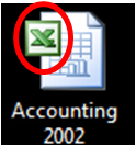
This icon belongs to Office 2007. If you take a good look at the small green Excel part of the icon you will notice that the upper right hand corner has been rounded. All previous versions of Office have all square corners as shown in the picture to the right.

Other New Features in Office 07

1. The toolbars have been replaced by Ribbons.
2. You can save as a PDF file by downloading a patch.
3. You can use more than three Conditional Formats.
4. Conditional Formatting presets have been added.
5. New Functions have been installed.
6. Quick Formatting for Tables have been added.
7. Quick Formatting for Charts and Graphs have been added under the Insert Tab.
8. On the Formulas Tab Functions Libraries have been added for quick use.

A look at the Main Workbook in Excel 2007

A look at the Main Workbook...
What is a Workbook?
Good Question, the workbook is Excels main document; it houses the Spreadsheets also sometimes called Worksheets.
The example below shows the Workbook, the main container of Excel. Inside of the Workbook there are three Spreadsheets. Three is the number of default Spreadsheets as designated by Microsoft.
A quick overview of the Microsoft Workbook Window, they will be explained in more detail later. For now I will give an overview.
Starting at the top left;












1. The Office Symbol, this is also a Command Button
2. The Quick Access Tool Bar (One of the two remaining tool bars left)
3. The Title Bar
4. Three Command Buttons
5. Back to the Left side of the screen, The Ribbon Headers
6. Groups
7. Title of the Group
8. Address Bar
9. Functions Dialog Bar
10. Select All Button
11. Now to the Spread Sheet, Column Headers (A, B, C…)
12. Running down the left side, Row Headers (1, 2, 3, …)
13. Cells
14. Move Buttons for the Spreadsheets
15. Tabs for the Spreadsheets
16. Slider bar For the Tabbed Spreadsheet
17. Status Bar

Link Excel 07 to PowerPoint 07

Things to keep in mind when linking a chart from excel into PowerPoint

1.       Save the excel workbook on the tab that the chart is on.  Otherwise it will not show the correct information.

2.       Unless you want to take the long way to copy and paste remember to check the Link checkbox.

Steps to linking the excel chart to PowerPoint

1.  Open the PowerPoint presentation that you wish to add the chart into.
2. Create a new blank slide.
3. On the blank Slide go to the Insert Tab and choose the Object button.
4. Make sure that you choose the Create From File choice.
5. Browse to the file location and choose the excel workbook you want.
6. Be sure to check the Link check box (otherwise you will have done the long way of copy paste).
7. Click OK.
8. Save the PowerPoint presentation and next time you open the presentation it will ask if you wish to update the link.  If you do click the Update Link button or if not click Cancel.

Excel Filtering 07

What does filtering do for me?

Filtering can help if you want to data mine, mine for information.  I can view my information by Males only and by SSG, or by Females and SSG. Anything that I want I can filter for as long as it is in my information.

Where to find the Filter Button?

You can find the Filter button on the Home Tab at the right hand side under Sort and Filter.

Set up Filtering

Click into your Labels row (Last Name, First Name, etc…)

Choose the Filter Button.

Drop Down arrows will appear in your Labels, in the lower right corner.

You can select what you wish to view by making sure that the check box has a check mark in it. The quickest way to uncheck everything is to click the (select all).

You may filter by as many criteria as you need.

Cautions when filtering

If you save the filtered workbook and open it again and you have not cleared the filters the information will still be filtered.  After the heart attack moment check to see

If the filter buttons are on

Are the Numbers to the left out of sequence and blue?

Is the filter button glowing orange/gold?

If the answer to any of these questions a yes, the filters are still turned on and the information is still filtered.

Excel Sorting

Things to be careful of when sorting

1.       If you choose the Column Header such a C, and then choose sort, you need to make sure that the choice Expand the Selection is selected or you will mix your record information up.

2.       If you click into an empty column and then try to sort nothing will happen.

3.       If you are outside of the range you will get an error message.

Normal Sorting

1.       Click into the information, a populated column, and click the sort button A to Z or Z to A depending on how you wish to sort.

a.        You can find the sort buttons on the Home Tab at the right hand side under Sort and Filter.

b.      Or you can find the Sort buttons on the Data Tab.

Custom Sorting Options

1.       Sort By: Gives a list of Column Headers that you can sort by.

2.       Sort On: Values, Cell Color, Font Color, Cell Icon.

a.       If you sort by Cell Color or Font Color you will need to create multiple sorts for the same column.  You can adjust the colors to fit how you wish them to be displayed.  Red then yellow then Green, Green then Red then Yellow.

3.       Order: A- Z, Z – A, Custom List

a.       Custom Lists will arrange the information in accordance to the specified list.  Sunday, Monday, Tuesday, Wednesday, Thursday, Friday, Saturday.

4.       My data has headers: Check box.

Custom Sorting

To sort by more than one field you need to choose Custom Sorting.  In combination with the above options you can sort various different ways.

1.       Click Add Level.

2.       Choose what column that you want to sort by.

3.       Choose what to sort on, Values being the most common.

4.       Choose how to sort, A – Z being the most common.

5.       Repeat as needed for as many criteria you wish to sort by.  (lather, rinse, repeat)

Excel Conditional formatting Office 07

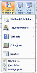
 Conditional formatting can be used to have Excel determine whether or not something falls within a specific guideline.  Say for instance that you want to track when someone needs retested, you could have the cell change color automatically depending on criteria.  The Conditional Formatting button is found on the Home Tab.  It has some prebuilt functionality, however if you need to you can create your own rules.

Conditional formatting for the example is as follows:

Notice the first line of the text is blue.  This has a conditional format associated with it that shows all the dates before 5/12/11 with a blue background.

              

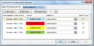
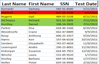
In order for us to show all of the information with the blue we need to be careful how we write the formula inside of the conditional formatting dialog.  Also, the placement of each rule is important here due to the fact that if I have the rules listed out of order the colors will be off.  For instance f I have the rule for 90 days out at the top all of the highlighted areas would be green not the rainbow as above.

If for some reason the formatting does not look correct on the Excel work sheet, when you have finished. It could be due to the fact that the Conditions are out of order, reopen the Conditional Formatting rules and make sure that the rule with the lowest value is at the top.  Another possibility is that the Cancel button was hit instead of the Apply or OK buttons.

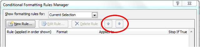
If for some reason the Blue does not appear  open the Condition Formatting Rules and move the blue rule up by using the arrows.  These conditional formatting rules should be at the bottom of the list.  We can move them by using the arrows in the upper right hand section of the Condition Formatting Rules Manager, see below.

Using the Today Function

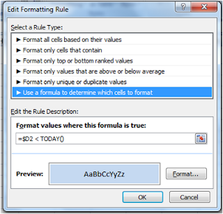
We will use the today function and compare it to cell D2 to get the required color.  In this case the formula would read; =$D2 < Today(). The next rule would be; =&D2 < Today()+30.  The third rule would be; =$D2 < Today()+60, and the last one is; =$D2 < Today()+90.

To conditionally format a single column of dates looking for 30, 60, and 90 days out.  Select the column header and go to the Conditional Formatting button, choose Manage Rules this will bring a dialog box up that we can use to create many different rules.  Click the New Rule button, another dialog box will appear.  Choose Format only cells that contain and fill in the information in the first dialog =Today() and the second dialog =Today()+30 this will select a date range for the next 30 days.  Format the cell fill color to red.

For the range of 60 days out we will want to make a second rule, click the New Rule button, another dialog box will appear.  Choose Format only cells that contain and fill in the information in the first dialog =Today()+31 and the second dialog =Today()+60 this will select a date range for the next 30 days.  Format the cell fill color to yellow.

For the range of 90 days out we will want to make a second rule, click the New Rule button, another dialog box will appear.  Choose Format only cells that contain and fill in the information in the first dialog =Today()+61 and the second dialog =Today()+90 this will select a date range for the next 30 days.  Format the cell fill color to green.

Alternating Cell Color

In order to create alternating row colors that will not move when sorted we can use conditional formatting.  These conditional formatting rules should be at the bottom of the list.  We can move them by using the arrows in the upper right hand section of the Condition Formatting Rules Manager, see below

If you wish to have alternating row colors, using conditional formatting, see image to the left.  We need to select the area that we wish to have the alternating lines of color.  I have chosen columns A to F and rows 1 to 19.

We need to go in to the conditional formatting Manage Rules and choose Use a formula to determine which cells to format.

In the Format values where this formula is true:, section we need to type in the following rule.

=mod(row(),2)=1

The =mod() means that we want to modify something, the selected area.

The row() or rows are what we are modifying.

The 2 tells Excel how many rows we are going to alternate the cell colors, see the example above.  Every two rows are colored.

The =1 tells Excel where to start the colorizing, in this case I started at row 1.  Our choices ore 0 (Zero) or 1, 0 starts at row 2 and 1 starts at row 1.